REN R 105 Exam 2

Gaia Hypothesis

Concept by Lovelock (1960s) and later with Lynn Margulis (1970s) that the Earth is a huge self-regulating system with homeostasis (temperature in a narrow range; two states of cool and warm, but still in a narrow range for life in past 3.6 Ga despite the sun’s intensity increasing by 25%)
Key is the presence of feedback loops (if too cold, feedbacks limit being colder and a shift to warm and vice versa)
Basically, inorganic, and organic components of the Earth are constantly in flux and interacting as a system
Widely criticized in the specific and analogy by some that Earth is a ‘living organism,’ but in the broadest sense, the general principles of interacting systems emerge in modern disciplines of systems ecology, biogeochemistry, etc.
A key message from the theory is that non-living and living world feed into one another, explaining why changes in one can have dramatic effects on the other
It also doesn’t mean that we don’t have to worry about anthropogenic climate change – Lovelock was very concerned about extra CO2 from humans pushing our planet beyond a threshold (Goldilocks zone)

Daisyworld Model

In response to critics, Lovelock and Andrew Watson created a model of a simple ‘planet’
-It is a planet with two species on its surface – white and black daisies
-The planet is not limited by water (rainfalls at night, days are clear)
-Water vapor and CO2 are assumed to be constant (no greenhouse effect)
-The key variable is that the two types of daises have different colors thus different albedos
-In a way, the daises can alter the temperature of the surface where they are grown via a negative feedback loop that maintains temperatures across a wide range of conditions
-A planet with dark soils and black daisies (low albedo → absorbs solar energy) warms planet, while white daisies (High albedo → reflects solar energy) cools planet
--Number of daises by species thus affects temperature
-Model assumptions: Daisies grow best at 25°C (die

Albedo

is a measure of the diffuse reflection of solar radiation out of the total solar radiation (0-1 scale)

Greenhouse Gases

Contribution of a gas to the greenhouse affect of radiative force is based on the characteristics of gas, its abundance, and indirect effects.
-For example, the radiative effect of a mass of methane is 84-times stronger than the same mass of carbon dioxide, but methane is present in much smaller concentrations so that its total direct radiative effect is smaller
Note that water vapour and clouds have large effects on climate (the biggest greenhouse effect), but it is not directly produced by humans and has short cycling times. Rather, H-2O vapor and clouds are ‘feedback’ variables in that they respond to climate warming (a warmer Earth can hold more atmospheric water vapor.
-Overall, water vapor’s contributes 50% towards the ‘greenhouse’ effect, clouds 25%, CO2¬ 20% and other gases 5%

Annual Greenhouse Gas Index

Most of the atmosphere is N2 (78%) and O2 (21%) with CO2 composition very low (0.04%, hence measured in ppm), but it has a big impact on warming as a greenhouse gas. It also has inertia/long cycling time (300-1000 years) meaning that even if human-related CO2 emissions stop now there will be inertia of future warning.
-Note that CO2 is growing much faster than other gases, so it is also having larger climate warming effects

Mauna Loa revisited

Since industrial revolution (the 1700s), CO2 concentrations have increased from about 275 ppm (ice core proxy) to 315 ppm in 1958 (start of direct measures) to 420 ppm today.
-Note that in the past 800 ka it typically ranged between 180 and 275 ppm

Global Surface Temperature

We are currently 1° to1.5°C over pre-industrial times, but it varies widely depending on the region of the planet (more extreme at high latitudes)
Note that there was a more noticeable increase in global temperatures starting in the late 1970s

Arctic Amplification

Climate warming has been greater at higher latitudes (also altitudes, but not shown here). This includes areas with warming as high as 4°C warmer in the current climate than 50 years prior
Why is Artic warming faster?
-It is thought to be mainly from positive feedback between sea ice melt and yet more warming of the air referred to as Artic amplification
How?
-Sea ice reflects the sun’s rays back into space (high albedo) reflecting more heat than it absorbs. This helps keep the Artic and planet cool.
-As sea ice decreases, there is more open ocean resulting in more heat absorption from the sun. As the ocean absorbs more heat, more ice melts thus creating positive feedback

Artic sea ice extent

September is when the ___ ______ is lowest
Note that the lowest recorded extents all within the past 10 years and much lower extent than the median extent over 30 years

Amplification of high-altitude climate warming

Although not quite as well-studied as the Artic, trends in climate warming at higher altitudes are also amplified
-For example, in the past 20 years temperatures above 4000 meters have warmed 75% faster than at altitudes below 2000 meters
How?
-The process is analogous to Artic ice but with respect to high-elevation late snow beds. Since snow reflects a lot of solar radiation (high albedo) if that snow melts with initial warming, more radiation gets absorbed by the ground thus heating the ground and warming the air. Current warming has shrunk alpine glaciers and ate snow beds amplifying the warming trend compared to prior times when snow was present

General Circulation Model

Much like current weather models, future climate models using – (sometimes called Global Climate Model).
-It is a model that employs mathematics of the general circulation of Earth’s atmosphere and/or oceans using Navier-Stokes equations on a rotating sphere with thermodynamics for energy sources (radiation, latent heat).
-These equations are the basis for simulating in a computer the Earth’s atmosphere and oceans.
-Are used for weather forecasting, understanding the climate and forecasting climate change

Regional Climate Model

Are also developed to isolate a single region of Earth & reduce complexity (often to allow finer resolution predictions)

Climate change pathways of SSP-RCOs from CMIP

Coupled Model Intercomparison Project (CMIP) is a framework to improve knowledge of climate change and modelling by the use of a standardized GCM framework.
Current models are CMIP6 of the 6th Assessment Report (AR6) of IPCC (Intergovernmental Panel on Climate Change)
Coupled models are computer-based models, like GCMs, of the earth’s climate in different parts (atmosphere, oceans, land, ice) that are “coupled” together and interact in simulations.
A number of different organizations output 40 CMIP model (UK, USA, Canada, etc.)
Representative Concentration Pathways (RCPs) assume different trajectories of greenhouse gas emissions & thus pathways for global climate change (radiative forcing). The most recent RCPs use SSPs (Shared Socioeconomic Pathways of RCPs as mitigation levels)

Representative Concentration Pathways

SSPs place the RCPs in language of socioeconomic narratives towards mitigating climate change gases

RCP 8.5

(warmest future, no mitigation) is characterized by increasing greenhouse gas emissions over time, representative of scenarios in the literature that lead to high greenhouse gas concentration levels

RCP 6

(moderate mitigation) is a stabilization scenario in which total radiative forcing is stabilized shortly after 2100, without overshoot, by the application of a range of technologies and strategies for reducing greenhouse gas emissions

RCP 4.5

(moderate mitigation) is a stabilization scenario in which total radiative forcing is stabilized shortly after 2100, without overshooting the long-run radiative forcing target level

RCP 2.6

(mitigation) is representative of scenarios in the literature that lead to low greenhouse gas concentration levels. It is a “peak-and-decline” scenario of greenhouse as emissions

Examples of projected climate change

Note that climate change models (GCMs) have greater accuracy in predictions of temperature than for precipitation. And average global temperature change is just that, an average
Some places (like the Artic) are projected to increase in temperature by 10°C by the end of the century

Forward Velocity

Is the rate to keep up with climate niche

Backward Velocity

Is from future climate back to matching current

Climate Change and Alberta's 'tree of life'

Non-random climate change risk to related plants (risk tends to be grouped phylogenetically)
Geographic patterns in gains and losses of 1541 plants in Alberta (climate niches)

Climate Change Refugia

Was originally used to represent the areas of stable paleoclimates or escape climates for species during historic times like the ice age (e.g., most species in Canada had refuge in the USA or Beringia).
However, in conservation ______ ______ is now also being used to examine where in the future places will be more stable, such as species where climate niches are still present in the same place.
Because there is geographic variation in the rate of climate change and species have different niches, there are distinct patterns in refugia
In this particular model, we considered the potential for migration with climate niches (birds certainly can migrate way faster than trees!)

Pleistocene Epoch of Quaternary Period

This most recent period we are in has substantially shaped the world, but especially so in Canada due to glaciers
2.58 Ma to 11.7 ka

Climate change in the past 420,000 years from ice core data

Glacial periods represented by low temps and low CO2
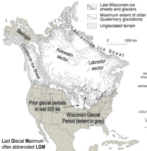
Five glacial periods in the past 500,000 years; most recent called the ‘Wisconsin Glaciation’
Likely four other global ice ages ranging from 260 Ma to 2.4 Ga (much less known about these old glacial periods vs. those within 500 ka)

Milankovitch Cycles and Earth's Climate

Orbital cycles:
-Eccentricity (100 k)
--Orbit shape
-Obliquity (41 k)
--Tilt
-Precession (26 k)
--Wobble
Theory: Variations in Earth’s Orbit (100,000 years), Tilt (41,000 years) and Wobble (26,000 years) affect incoming solar radiation and thus help start and end ice ages

Distribution of glaciers in last 1 Ma (N. Hemisphere)

Southern hemisphere is home to the large Antarctica Ice sheet, but then much smaller historic ice sheets in Patagonia to Andes, New Zealand, etc.

Ice Volume and sea levels

North America had by far the largest glaciers in extent and volume
As water is locked up in glaciers, the sea levels fall (in the last Wisconsin glaciation, sea levels were 120m lower resulting in land bridges etc.)

Global extent of glaciers at 20 Ka (peak of Wisconsin Glaciation)

North America had the largest glacial extent besides Antarctica
Much of Asia, including Siberia to Yukon, was free of ice (presumably too dry) – an area called Beringia
Some parts of Beringia have been ice-free for 1 Ma
Last Glacial Maximum – In white
Most recent Wisconsin Ice Sheet (grey edges slightly less south)
-Cordilleran Ice Sheet (Mountains)
-Laurentide Ice Sheet (Keewatin and Labrador sectors)

Remaining Continental Glaciers

Antarctic and Greenland Ice sheets

Post-glacial isostatic adjustment

How fast the crust pushes back up

Isostatic Rebound: Great Lakes example

Total rebound north of the Great Lakes toward the Hudson bay is substantial (100s of metres and not finished yet)
Ice compressed the land surface like a sponge or marshmallow springing back

Ice-free Beringia

Much of Siberia and northern Alaska and Yukon was unglaciated, thus refugia for megafauna

North American Ice-Free Corridor (IFC)

Has been a focus of research:
-Open ___ by ~13.8 ka (+/- 0.5 ka)
-Beringia was ice-free in the north, humans and wildlife migrating from Asia to ice-free areas in the south were blocked by glaciers
-Recent work suggests the opening as later than fossil human evidence further south (15.6 ka) suggesting a coastal route was first
As the glacier receded large glacial lakes called Proglacial Lakes would form at their margin
Some of these were among the largest known lakes to ever occur on Earth (e.g., Glacial Lake Agassi)
In many cases lakes would drain rapidly as isostatic rebound ‘pushed’ water over divides or ice dams broke thus cutting glacial spillways valleys over days or weeks with ‘misfit’ streams now occupying their massive valleys
-Small streams in big valleys

Glacial Lake Agassiz

Proglacial Lake ~285,000 km2 in area, it covered most of what is now Manitoba and parts of Saskatchewan, Ontario, North Dakota and Minnesota
Extent over multiple time periods (it was never that large at any one time)
Multiple ‘mega floods’ occurred draining the lake and cutting ‘spillway’ river valleys
Some speculate that the last draining of Lake Agassiz to Hudson Bay put so much cold, freshwater into the Atlantic that it temporarily slowed the North Atlantic Current cooling Europe for centuries

Alberta's connection to lake Agassiz mega-flood

Clearwater to Athabasca to Artic Ocean (NW route)
Mega flood thought to have lasted ~78 days, 9.9 ka
Cut the Clearwater gorge
Massive deposits of delta sands 100s km downriver

Western North America Mega-flood

Glacial lake Missoula and Columbia → Channeled Scablands of E. Wash
Camas prairie, sand ripples up to 9m high (like you would see at small scales at a beach; i.e. scale variance)
Flood is thought to be dated between 15 to 13 ka (likely multiple floods, but possibly one large one
Water depth estimated at ~120m at the site
Water estimated to be flowing at 105 km/hr
Water volume: 10x all the Earth’s current rivers
Think Niagara Falls as smaller example
Some suggest that if the flood lasted much longer (i.e., hours to days), the Umatilla Rock fluting would have eroded away

Potholes

Formed from extreme vortexes in the water

Catastrophism vs. Uniformitarianism

Competing geological theories

Mega-floods and sea level rise

________ may help explain rapid ____ ___ _____
Pulse 1A is likely from Mississippi basin deglaciation (floods), while 1B is from more northern and western floods of the Younger Dryas.
Regardless, we are talking 50m sea level rise over a short period and 120m since the last glaciation

Younger Dryas was a time of rapid change

Period: 13.9 to 11.7 ka
11.7 ka is considered the end of the ice age
Named after an artic plant (_____ octopetala) showing up in Europe’s paleo-vegetation (pollen) at this time (cold period)
Much debate on what initiated the dramatic cooling at 12.9 ka and the dramatic warming at 11.7 ka

A black ‘mat’ dated to the Younger Dryas period

Many sites in North America and Europe with a black ‘mat’ layer in the soil horizon dating to Younger Dryas
No evidence of megafauna within or above this horizon (younger period [soil horizons] after YD)

Magnetic particles and microspherules inside the black mat

Microspherules are known to form at >2,200°C comparable with cosmic impact material from Meteor Crater, Arizona, and material from the Trinity nuclear airburst in Socorro, New Mexico
Inconsistent with anthropogenic and volcanic materials, suggests molten iron droplets
Examples found at eighteen widely separated site by Wittke et al. (2013) dated to 12.8 Ka (start of YD)

Younger Dryas impact theory

Highly debated theory (some folks totally disagree)
If it was Extra Terrestrial (comet) it likely broke up in space hitting multiple sites
If an ET, it helps explain mega floods and megafauna loss
Smoking gun and impact(s) sites missing (could have hit the ice sheet itself, but candidate sites provided like Northern USA (Michigan), Canada and Greenland (secondary impacts elsewhere
Orientation places original impact near Great Lakes 1500km away
-Similar structures in Nebraska also point to Great Lakes
Craters point to Michigan, which at 12.8 ka would have been ice covered (sending massive ice boulders 100s of kms)
-Controversial idea

Carolina Bays

Inferred to be 'ejecta' craters (secondary impacts by ice)

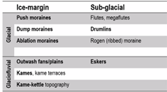
Continental glacier landforms

Glacial landforms in mountains have their own terminology

Drumlins and Fluting

All agree that _______ originate “under” the ice (subglacial) but originally believed to be actions of ice scouring of material
More recent suggestions are these were developed under the ice through fluvial (flowing water) in massive floods
100+ years of study we are still unsure

Glacial Erratic

Large rocks from elsewhere (obvious different geology); used to be call “drift” by geologists prior to late 1800s (assumed to be rocks in melted icebergs in ancient ocean dropping rocks on land below)

Glaciolacustrine

Glacial lake deposits

Glaciofluvial

Glacial river deposits

Surface geology

Refers to the unconsolidated geologic materials lying on top of the bedrock. Generally referring to glacial (Quaternary) deposits

Stagnant Ice Moraine

Collapsed and slumping of debris near ice margin ~20km north of Tofield.
‘Doughnuts’ are classic stagnant (dead) ice features
-Doughnut features
--Sediment fills hole in low ice
--Sediment slumps down trapping ice (insulating)
--Ice melts slumping the middle down
Not a few flat topped kames (also called ‘perched lake plain’ or ‘ice-walled lake’ because of how they were formed)

Surficial deposits of Alberta

Glaciolacustrine
Glaciofluvial
Eolian deposits
Drumlin and Kame
Stagnant Ice Moraine
Ice-thrust Moraine
Major meltwater channel

Ice-thrust Moraine

Till formed displacement of block or 'rafts' that are left more less intact

Major meltwater channnel

Massive river drainage during melting of glacier and possible major break in glacial lake
In many areas you will not an ‘undersized’ (misfit) stream in a massive valley pointing to past carving of the channel

Why is all of this important?

Canada’s landscapes were very much shaped by our recent glaciers
Different deposits results in different environmental resources (aquifers, agriculture/soils, gravel, species habitat) and sensitivities (to pollution, to climate change, to land cover change)
Understanding the history and landforms is fundamental to understanding our environment

Key events in the history of life

3.7 Ga: life’s simple molecules
3 Ga: prokaryotic cells
2.5 Ga: first eukaryotic cells (single cells)
1.5 Ga: first multi-cellular organisms
575 Ma: ‘complex’ life evolves (Cambrian explosion etc.)

Tree of life

Charles Darwin and Ernst Haeckel

Hydrothermal vent theory

Life 3.8 Ga came from harnessing energy gradients when alkaline vents water mixes with more acidic seawater (early oceans were more acidic); some suggest geothermal vents on land, panspermia, etc.
These vents had mineral pores that were templates for cells separating vent and sea water
These mineral membranes mirror the way that cells harness energy vis a proton gradient (pumping protons across a membrane to create a charge; called the proton-motive force – 3 pH unit difference)
This provided a mechanism to store potential energy with energy harness with protons were passed through membrane (ADP to ATP – energy used for powering life)

Life as a single cell

The first 1 Ga of life contained ONLY bacteria and archaea representing two of the three genealogical branches of the tree of life
The lowest groups on the tree of life, including thermatogales and most archaea, are anaerobic organisms
Key even in evolution was the invention of photosynthesis (3.5 Ga) and cyanobacteria (2.7 Ga) making oxygen and now forming the base of our planet’s energy flow
First eukaryotic cells (still single celled) evolved 1.7 to 2.5 Ga, perhaps coincident with rise in atmospheric oxygen 2.3 Ga
Throughout the Proterozoic era, from about 2.3 Ga until 575 Ma, life on Earth was mostly single-celled. Earth’s biota consisted of bacteria, archaea and eukaryotic algae

Archaea

Microscopic single-celled organisms

Anaerobic organisms

Cannot tolerate oxygen, early Earth had no atmospheric oxygen so life used hydrogen, sulfur, or other chemicals for energy

Endosymbiosis Hypothesis

All eukaryotic cells have organelles: sub-components with specialized functions (e.g., assemble proteins, digesting food)
In plant and eukaryotic algae cells, chloroplasts carry out photosynthesis; these organelles represent aerobic bacteria that took up residence inside host cells and carried out photosynthesis there (another key endosymbiont event)
Margulis

Mitochondria

The organelles that conduct cellular respiration (Converting energy into usable forms) in eukaryotic cells were descended from cyanobacteria providing energy in cells (endosymbiosis)

Endosymbiosis

Now the tree of life becomes more complicated and not really a true ‘tree’ with branches that cross over between major domains and in some instances explaining entire new groups of life (e.g., plants)
Symbiosis (in some cases ‘serial’ symbiosis was critical to development of ‘complex’ life and only happened a few times in its history despite massive amounts of time (3.8 Ga)

Horizontal Gene Transfer

Process in which prokaryotes also are now known to share their genes
This is defined as the introduction of genetic material from one species to another species by mechanisms other than the vertical transmission (evolution) from parent(s) to offspring.
These transfers allow even distantly related species to share genes, influencing their phenotypes
Three types of ____________ ____ ________
-(1) Conjugation (from another bacterium)
-(2) Transduction (from bacterial virus)
-(3) Transformation (from the environment)

"Web of life"

Symbiosis and Horizontal Gene Transfer means that there is cross-over that complicates the tree of life and provides key inventions

Modern Phylogenetic Trees

Can be shown as circular, rectangular divisions, or tree-like
The basal root or start is called LUCA

LUCA

Last Universal Common Ancestor

Witnessing evolution in real-time

Long-term (1988-present) evolutionary experiment of genetic changes in twelve initially identical populations of asexual Escherichia coli (E. coli) bacteria
Grows more that six generations/day – equivalents of more than 150 years of human history
Each day, 0.1 milliliter from each 10-milliliter flask is transferred to a new flask filled with water and sugar and allow to multiply; repeated
Every 500 generations (75 days), a sample from each population is stored in a super-cold freezer
They then compete the current with historic generation (grown next to each other) to see how much faster each of the 12 populations reproduces compared with its ancestors
Billions of genetic changes have occurred during the experiment (every single letter of the DNA’s 4.6 million base pair has been mutated multiple times); some rare mutations have been successful (new generations reproduce 70% faster)

Natural Selection via a power law

A key finding was that natural selection (fitness) did not asymptote despite the same environment (food source, temperature). Initial idea was that evolution may asymptote without environmental changes. (hypermutator populations even higher continual growth)

Natural selection via an important mutation

One flask turned opaque overnight in 2003, clouded by a sudden overgrowth of bacteria. Somehow, the microbes inside were growing faster. They found that the bacteria evolved the ability to ear the citrate added to their flasks to help them ingest iron (bacteria could now access new stores of energy previously out of reach)

Antibiotic resistance of bacteria has evolved

Note antibiotic use, particularly in livestock is leading to antibiotic resistance. Just within the USA alone, farmers used 6.1 million kilograms of medically important antibiotics in 2019, this is a problem for human health

Variation

There is genetic variation within a population (mutations, etc.)

Competition and differential survival

Over-production of off-spring leads to competition for survival

Adaptation

Individual with beneficial adaptations are more likely to survive and pass on genes

Selection

Over many generation there is a change in allele frequency (evolution)

Evolution of Sex

Invention of sex 2 Ga supercharged evolution (99.9% of eukaryotes today do it) allowing rapid diversification and adaptation of species to changing environments
Some debate about advantages/disadvantages of sex and Darwin’s analogy, but overall when environments are variable and species compete, sex can be advantageous (but, remember that bacteria have other mechanisms lift HGT to overcome this limitation

Tangled Bank Hypothesis

Darwin proposes that sex evolved to prepare offspring for the world around them (Darwin refers to a wide assortment of creatures all competing for light and food on a ‘_____’ and competition necessitates rapid evolution via sex)

Red Queen Hypothesis

First proposed by Leigh Van Valen in 1973
States that species must constantly adapt, evolve and proliferate to survive while pitted against ever-evolving opposing species
Challenger to the Tangled Bank hypothesis (for ‘why’ sex)
Implication is that predator and prey (host-parasite) must be constantly evolving to avoid extinction (evolutionary arms race)

Natural Selection drives speciation and thus biodiversity

Natural Selection can lead to speciation, where one species gives rise to a new and distinctly different species, particularly in the presence of geographic and environmental variability
Helps explain the diversity of life on Earth

Biosphere

Identified by Eduard Suess in 1875, which he defined as the place on Earth’s surface where life dwells
In practical terms, the _______ is the worldwide sum of all living organisms (biota or biomass), but also defined as ‘systems’ (ecosystems) that are closed and self-regulating (similar type of vegetation and species)

Biomass Proxy

In aquatic systems, chlorophyll production is a good proxy of biomass even if only measuring the trophic base (plants).
On land, remote sensing methods of NDVI (Normalized Difference Vegetation Index) quantifies the amount of green plants present on the land surface based on ration of Near infrared to infrared remote sensing
-Yellow-brown scale are deserts; blue-green is high

Holdridge's Life Zone Concept (1947)

Three axes (subdivisions) are based on:
-Precipitation (annual, logarithmic)
-Biotemperature (mean annual, logarithmic)
-Potential evapotranspiration ratio (PET) to mean total annual precipitation
Additional indicators include:
-Humidity provinces
-Latitudinal regions
-Altitudinal belts

Whittaker’s Biome concept of ecosystems

Has a number of important ecological and biological contributions in the 1950s-70s
-For example in 1969 he proposed five kingdom taxonomic classification of the world’s biota (Animalia, Plantae, Fungi, Protista and Monera)
-In ecology, he developed, among other things, a biome classification of the world’s ecosystems in 1962 using simple, but important climate variables of mean annual precipitation (MAP) and temperature (MAT)

Whittaker's "Ecosystem uncertain"

The map shows the areas that contain non-forested conditions despite being suitable climatically to grow trees
So, what limits tree growth? Well, in areas of the world where temperatures are suitable for trees, it would be precipitation (or available moisture).
Where moisture is limiting then that limits trees & the
actual biomass is similar to the potential biomass
(also at the boundary to another biome of
grasslands).
William Bond (2005) suggested a solution to this question saying that large areas of the world are ‘consumer-controlled’ and specifically via two mechanisms: 1) large mammals as biotic consumers (note, however, massive ‘recent’ extinctions in late Pleistocene); and 2) fire as an abiotic consumer (many analogies to herbivory)
Others have suggested ‘resource constraints’ (Like soil nutrient limitations) that explain open conditions, but it does not explain the broad extent of ecosystem uncertain like Bond’s consumer-controlled hypothesis

Ecosystem uncertain

Vast areas of non-forested vegetation occur where climates are suitable for forests.

Ecoregions further divide the biome concept

The ecoregion concept adds information on local soils, landforms since climate alone doesn’t fully sub-divide local ecosystems
For instance, the boreal forest is quite large with local differences in forest types that depend largely on the substrate (e.g., Canadian Shield, outwash sands, peatlands)
In North America, one commonly used map uses hierarchal classification (three nested ‘levels’)
-Level 1 has 15 broad types
-Level 2 has 50 types subdividing the 15
-Level 3 of 182 types

Example: Temperate deciduous forests

Temperature forest ecosystem (species) began to appear in fossil floras from the Late Cretaceous (66 Ma)
Note locations of ‘temperate’ conditions at the time were more toward the poles because climates were warmer at that time
Temperate forest ecosystems became more ‘disjunct’ over time to what we have today

Disjunct genera between E. NA and E. A

Two regions have similar climates today and as well as in the past when continents were nearby
Large number of genera are shared between the areas (trees most widely studied)
More recent comparisons show Eastern North America is more like Western North America, but that Eastern Asia is more life Eastern North America than Western North America despite being closer

Gray's Hypothesis

Asa Gray (botanist in the 1800s) compared flora of Eastern North America to Western North America to Eastern Asia suggesting that a closer relationship between Eastern Asia and Eastern North America than Eastern North America to Western North America

Glacial refugia - Example western trees

Western refugia was more complicated because of the complexity of mountains, deserts, etc. but some key ecosystems considered as refugia (not also Alaska Beringia)

Reid's paradox of Holocene plant migration

Is the mismatch in theoretical estimates of invasion rates and observed rates of migration, particularly in the Holocene postglacial migration
Named after Clement Reid, a paleobotanist, who observed (1899) that palaeobotanical records of oaks in Europe that the rate of migration was more rapid than predicted (birds likely long-range seed dispersal)
While Reid couched his paradox in terms of the migrations of oaks in Great Britain, same phenomenon in a wide variety of species. In almost all cases, these authors suggest that occasional, long-distance events, probably due to active dispersal factors (ants, birds, rodents) are responsible
But also note that comparing current migration within existing communities is different than migrating the recent barren ground (no competitors)

Example of Reid's paradox

Despite seed size of oaks (Quercus) being much larger than other Eastern Deciduous Forest species, it managed to migrate back post-glaciation faster than many others

Rapport's Rule

Range sizes of plants and animals increase with latitude (large at high latitude, smaller at lower latitude)

Bergmann's Rule

Body size of animals increase in colder environments (vs. smaller in warmer), thus body size increases with latitude

Range Limits

Of species differ at high latitude limit (abiotic factors – climate limitations) to lower latitude limits (biotic factors – competition)

Biogeographic rules of species distribution

Rapport's Rule
Bergmann's Rule
Range limits

Grinnellian Niches

Is the ecological role of a species. It specifically refers to the habitat in which a species lives and its accompanying behavioural adaptations
Here the niche is the sum of the habitat requirements and behaviours that allow a species to persist and produce offspring.
It has been described as the “needs” niches, or an area that meets the environmental requirements (needs) for an organism’s survival

Eltonian Niche

Is the species’ place in the biotic environment, its relations to food and enemies
Elton classified niches of animals according to foraging activities (food habits)
Example: a carnivore niche (each ecosystem would have a type of carnivore in the food web even if the species differs)
This niche concept does NOT focus on individual species like the other two concepts