Module 12 - Two-factor ANOVA

Two-factor ANOVA

Used to evaluate the change in a numerical variable across two categorical variables. Builds on the single-factor ANOVA, can look at the effect that each level has on the numerical variable and the interaction between categorical variables

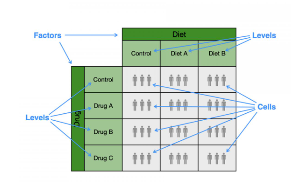
Structure of a two-factor ANOVA

Can be visualized as a two-dimensional grid. One factor can be columns and the other rows

Main effects

Answered in a two-factor ANOVA — can be for factor A: asking about differences among the levels of factor B. These are comparisons among full columns (or full rows) AND for factor B: asking about the differences among the levels of factor B averaging across the levels of factor A. These are comparisons among full rows (or full columns).

Interactions

Questions about the differences among the levels of one factor within each level of the other factor. These are cell-bycell comparisons.

Evaluation of if there is an interaction between the factors

Asks if there is an interaction — any deviation from the assumption that the levels of each factor simply add together (additivity)

Assumption of additivity

The response to the combination of two levels is simply the sum of the two — ie. stacking two 1kg rocks on a scale will result in a measurement of 2kg

Interaction plot

A common way to visualize data - a specialized plot that highlights the interaction pattern between two categorical variables. Use the same information as a box plot but presents the data in a way that showcases the relationship.

Setup for an interaction plot

1. The y-axis shows the numerical variable in the same way as box plots

2. The x-axis shows the levels one categorical variable

3. Lines are used to connect cells across the x-axis according to the levels of the other categorical variable

Representation of categorical variables on an interaction plot

If the categorical variables are additive (no interaction), the lines will be parallel. If the categorical variables are not additive, the lines are not parallel. Antagonistic interactions have lines that cross. Synergistic interactions have non-parallel lines that don’t cross

Null and alternative hypotheses for main effects (ie., A)

Null: The means (μ_Ai) are the same across all levels (i) of factor A: H_O: μ_A1=μ_A2=...=μ_Ak-1=μ_Ak

Alternative: The means are different somewhere: H_A: μ_A1≠μ_A2≠...≠μ_Ak-1≠μ_Ak

Null and alternative hypotheses for interaction

Null: the deviation of each cell relative to additivity is zero (notation A_iB_j refers to the cell that corresponds to the ith level of factor A and the jth level of factor B): H_O: δ_A1B1=δ_A1B2=...=δ_AkBk-1=δ_AkBk=0

Alternative: There is a non-zero deviation from additivity. Does not indicate which cells or how many have non-zero deviations. H_A: δ_A1B1≠δ_A1B2≠...≠δ_AkBk-1≠δ_AkBk≠0

Group variation factor A (MS_A)

The variation among the means of the levels of factor A. Calculated as MS_A=SS_A/df_A, where SS_A is the total group variation and df_A is the degrees of freedom. Degrees of freedom are df_A= a-1, where a is the number of levels in factor A.

Group Variation factor B (MS_B)

The variation among the means of the levels of factor B. Calculated as MS_B=SS_B/df_B, where SS_B is the total group variation and df_B is the degrees of freedom. Degrees of freedom are df_B= b-1, where b is the number of levels in factor B.

AB interaction (MS_AB)

The amount of variation attributable to the deviation from additivity. Calculated as MS_AB=SS_AB/df_AB, where SS_AB is the total variation of the cell deviations from additivity and df_AB is the degrees of freedom. Degrees of freedom are df_AB= (a-1)(b-1), where a is the number of levels in factor A and b is the number of levels in factor B.

Residual Variation (MS_E)

The variation among sampling units within a cell. Calculated as MS_E=SS_E/df_E, where SS_E is the total residual variation and df_E is the degrees of freedom. Degrees of freedom are df_E= ab(n-1), where a is the number of levels in factor A, b is the number of levels in factor B and n is the number of sampling units in each cell.

Three F-tests

Main effects A/B: (ie. A) The F-score is F=MS_A/MS_E, where MS_A is the group variation for factor A and MS_E is the residual variation. This ratio of variances evaluates mean differences among factor A levels by quantifying the amount of factor A group variation relative to residual variation.

Interactions: The F-score is F=MS_AB/MS_E, where MS_AB is the cell variation attributed to non-additivity and MS_E is the residual variation. This ratio of variances evaluates an interaction by quantifying the amount of variation attributable to deviations from additivity relative to residual variation.

Scientific conclusions for a two-factor ANOVA

First: Evaluate the interaction, either:

1. Reject the null hypothesis and conclude there is evidence that at least one cell deviates from additivity.

2. Fail to reject the null hypothesis and conclude there is no evidence that the cells deviate from additivity.

If to reject the null hypothesis, main effects should not be evaluates (the presence of interactions says the change in means across levels of one factor differs depending on the level of the other factor)

Second: Evaluate the main effects, if the interaction is not significant, factors are considered additive, can look at main effects for each and conclude:

1. Reject the null hypothesis and conclude there is evidence that the means of at least two levels are different in the factor.

2. Fail to reject the null hypothesis and conclude there is no evidence that the means among levels are different in the factor.