Beanie Exam 7

Good luck handsome!

Benktander Pros and Cons

• Advantages

  • BG MSE is almost always smaller than BF or CL

    • BG MSE is almost as small as the optimal credibility reserve

  • Better approximation of the exact Bayesian procedure

  • Superior to CL since it gives more weight to the a priori expectation of ultimate losses

  • Superior to BF since it gives more weight to actual loss experience

• Disadvantages

  • Requires an a priori estimate of ultimate losses

Benktander: if c* > p_k / 2

 then BG reserve has a smaller MSE than BF reserve

Benktander: Esa Hovinen Reserve

R_eh = c * R_cl + (1-c) * R_bf

If c = p_k then R_eh = R_gb

Benktander: Chain Ladder Ultimate Formula

Hurlimann ELR

• If using BF 🡪 Use the selected LDF and A Priori estimates

• If using Cape Code 🡪 Calculate ELR using age-to-age factors instead of calculating mk and pi

  • Sum (latest diagonal loss figures) / sum(used premium)

Hurlimann Individual Resersve

Hurlimann Collective Reserve

ADVANTAGE OVER BF: BASED ON OBJECTIVE DATA

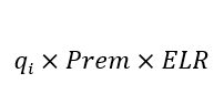
HURLIMANN BENKTANDER CREDIBILITY

HURLIMANN NEUHAUS CREDIBILITY

ASSUMES CONSTANT ELR

HURLIMANN OPTIMAL CREDIBILITY

HURLIMANN - Z_opt, t_opt, f_i

HURLIMANN

HURLIMANN

HURLIMANN

Optimal weights minimize MSE between estimated & true reserves → closest to 1 is optimal

HURLIMANN

BROSIUS - LEAST SQUARES PROS

• Advantages

  • More flexible than link ratio (CL), budgeted loss (ELR), and BF methods

  • Places more (or less) credibility on the loss experience as appropriate

  • Produces more reasonable results when data has severe random, year-to-year fluctuations

BROSIUS - LEAST SQUARES METHOD

• Use =SLOPE & =INTERCEPT to calculate the ult loss ratio by AY, iteratively 🡪

  • Start with more mature AY’s to add more data points in later iterations of the process

• Assumes no systematic shifts in the book of business

  • If significant premium growth 🡪 convert losses to Loss Ratios

  • Adjust incurred loss data for inflation so all AY’s are on a constant-dollar basis

  • If there is significant growth in the book of business, you should divide by an exposure basis

• INTERCEPT < 0, use the link ratio (CL) method

• SLOPE < 0, use the budgeted loss (ELR) method

BROSIUS - CREDIBILITY ON THE LINK RATIO

BROSIUS - HUGH WHITE’S QUESTION

If reported losses come in higher than expected,

• Budgeted Loss method – reserve estimate will decrease but ultimate loss stays the same

• BF Method – reserve does not change; ultimate loss increases by difference in actual and expected loss

• Link Ratio – ultimate loss estimate increases in proportion to the excess losses by applying the LDF

BROSIUS - LINEAR APPROXIMATION

RESERVE = X - L(x)

BROSIUS - LINEAR APPROXIMATION - HOW LARGE LOSS CAN CHANGE THE LOSS RESERVES

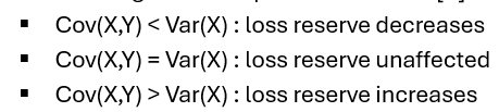
BROSIUS - LINEAR APPROXIMATION KEY POINT

THE LEAST SQUARES METHOD IS THE BEST LINEAR APPROX TO THE BAYESIAN ESTIMATE

BROSIUS - LINEAR APPROXIMATION ADVANTAGES

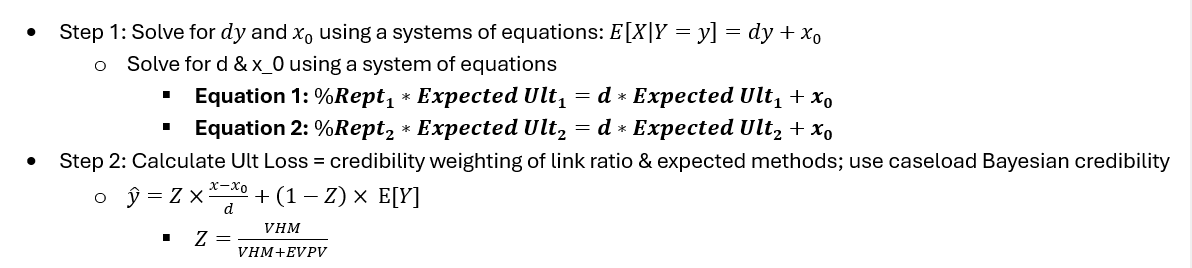
BROSIUS - BAYESIAN CREDIBILITY IN A CHANGING SYSTEM

BROSIUS - BAYSEIAN CREDIBILITY IS APPROPRIATE FOR

• A NEW LINE OF BUSINESS

• THERE IS A CHANGE IN THE BOOK MOVING FORWARD

BROSIUS - CASELOAD EFFECT

FRIEDLAND (REINSURANCE) - REINSURANCE STAKEHOLDERS

• Internal management – sound reserves affect all areas of reinsurer operations (pricing, underwriting, strategic planning, financial decision-making, etc.)

• Investors – appropriately stated reserves are essential so that investors can properly evaluate the reinsurer’s balance sheets and income statements for their decision-making

• Insurance regulators – regulators rely on the financial statements of reinsurers to properly supervise the reinsurance market

• Rating agencies – if a reinsurer reports significant adverse reverse developments over time that reduce capital leaving the reinsurer in a weakened position, it could face a rating downgrade

FRIEDLAND (REINSURANCE) - FUNCTIONS OF REINSURANCE

• Promote stability – ceding company stabilizes its loss experience; decreased proability of ruin

• Increase capacity – by ceding, a company increases capacity to write more business / high limit policies 

• Protect against CATs – protect ceding companies from CATs & casualty loss occurrences w/ multiple insureds

• Manage Capital and Solvency Margin

  • Pass risk of large losses to the reinsurer 🡪 frees capital since less is required to support policies written

  • Ceded commission acts as a transfer of statutory surplus to the cedant from the reinsurer

  • Ceded premium reduces cedant net premium-to-surplus ratio, allowing them to write more business

• Access technical expertise – reinsurers have expertise in underwriting, marketing, claims, prevention, pricing

• Other functions – withdrawing from a line of business, geographic area, or production source

FRIEDLAND (REINSURANCE) - TYPES OF REINSURANCE: HOW THEY WORK - TREATY

• Cede all business arising from LOBs that fall within terms of the treaty subject to treaty limits

• No underwriting by reinsurer of individual risks

• Cedant obliges to cede risk under the treaty terms;  reinsurer obliges to automatically accept it

FRIEDLAND (REINSURANCE) - TYPES OF REINSURANCE: HOW THEY WORK - FACULTATIVE

• Cedant and reinsurer have the option (faculty) to accept/reject individual submissions

• Each policy has their own negotiated agreement

• Primarily used to increase capacity, typically for high-value and hazardous commercial risks

  • Facultative automatic – a bordereau of risks ceded is submitted to the reinsurer, which has limited rights to decline individual risks

  • Facultative obligatory treaty – a treaty under which the cedant has the option to cede or not cede individual risks. The reinsurer must accept any risks that are ceded

FRIEDLAND (REINSURANCE) - TYPES OF REINSURANCE: HOW THEY WORK - PROPORTIONAL

• Increases capacity & manages capital and solvency margins to provide surplus relief

• Premiums & losses shared based on cession percentage.

• The reinsurer pays a ceding commission to reimburse cedant for expenses underlying the policy

• Types

  • Quota share – agreed % of each risk is ceded for the LOBs included in the treaty

  • Surplus share – cede the surplus amount of risk above the retained line subject to maximum ceded % and limit

FRIEDLAND (REINSURANCE) - TYPES OF REINSURANCE: HOW THEY WORK - NON - PROPORTIONAL

• Provides stability by protecting losses above a limit for risks ceded

• Loss ceded based on size of loss and premium is not proportional

• Types

  • Excess per Risk – excess of loss above a retention for each risk

  • Excess per Occurrence – protects from accumulation of loss from single occurrence

  • Excess per CAT – protects from accumulation of loss from single CAT

  • Annual Aggregate Excess of Loss (Stop-Loss) – cedant loss won’t exceed a threshold

  • Clash – attaches above all other policy limits; Protects against multiple claims from multiple insureds

    • Components of a clash event

      • Loss must have multiple policies by one insured or similar policies held by multiple insureds

      • Losses are traceable to and the direct consequence of a specific event

      • Event takes place within a specific timeframe

FRIEDLAND (REINSURANCE) - TYPES OF REINSURANCE: HOW THEY WORK - FINITE RISK REINSURANCE

• Features include:

  • Risk transfer and risk financing in a multi-year contract

  • Incorporates the time value of money and investment income

  • Limited assumption of risk by the reinsurer

  • Reinsurer and ceding company share results

• Includes run-off solutions, which transfer reserve development risk to the reinsurer. Reasons for run-off include

  • Corporate restructuring

  • Mergers & acquisitions

  • Discontinuations of lines of business

  • Erratic changes in the valuation/cost of a liability

• Loss portfolio transfers

  • transfers all (or portion) of liability for future loss payments on losses already incurred

  • relieves cedent of uncertainty in loss reserves and relieves capital

• Adverse development cover 

  • ceding company is reimbursed for losses excess a retention but no transfer of the loss reserves to the reinsurer

  • often used for M&A to transfer the risks of timing and adverse reserve development

FRIEDLAND (REINSURANCE) - REINSURANCE CONCEPTS & CONTRACT PROVISIONS

• Inure to the benefit of – determine the ordering of the contracts

• Losses occurring during vs risks-attaching – determines coverage

• Subscription percentage – reinsurance policy where risk is shared by multiple reinsurers, each of whom have a subscription percentage

  • Allows diversification of credit risk

  • Coverage may be more than one reinsurer is willing to assume

• Commutation clause – ending reinsurance contract early

FRIEDLAND (REINSURANCE) - REASONS FOR COMMUTATION

• Cedant

  • Exit LOB

  • Manage reserve for transfer or sale

  • Avoid credit risk of reinsurer

  • Better manage claims and claims-related expenses

• Reinsurer

  • Terminate relationships with cedants

  • Protect from insolvency of a cedant

  • Avoid dispute with cedant about future loss development

FRIEDLAND (REINSURANCE) - SUFFICIENCY, RELIABILITY, DATA CHALLENGES

• Sufficiency – data includes all info needed for actuarial work

• Reliability – data is sufficiently complete, consistent, and accurate for the purposes of the work

  • Data should be validated and reviewed for consistency, completeness and accuracy

  • Challenges

    • Influence of change in operations and environment

      • operational changes for ceding insurers and reinsurers

      • changes in legal/economic environment of ceding companies that impact loss

    • Different IT systems, terminology

    • Reporting lags & gaps in reporting

    • Manuscript nature of reinsurance policies

      • contract wording can be different by contract making it difficult to aggregate data

    • Other experience typically excluded

      • run-off data

FRIEDLAND (REINSURANCE) - HOMOGENEITY AND CREDIBILITY DATA

DATA SHOULD BE SEGMENTED INTO GROUPS WITH SIMILAR CHARACTERISTICS OF LOSS EXPERIENCE SUCH AS COVERAGE, REPORTING, SEVERITY, AND VOLUME

FRIEDLAND (REINSURANCE) - COMPARISON OF DEVELOPMENT FACTORS & PATTERNS (IN TERMS OF VOLATILITY)

• Reinsurance > Primary at earlier maturities

• Paid > Reported for Reinsurance business

  • Due to longer reporting/payment patterns for reinsurance b/c of lags in reporting to the reinsurer

• Non-Proportional Treat & Facultative > Proportional treaty

  • Greater volatility means greater uncertainty in projected ultimate using development method

• CAT > Ex CAT

  • Development methods are often not appropriate for CATs

FRIEDLAND (REINSURANCE) - IMPLICATIONS OF VOLATILITY IN LOSS DEVELOPMENT

• Greater volatility in projected Ultimate loss results in greater range in indicated IBNR and Total Unpaid for

  • Reinsurance compared to primary

  • Non-proportional & fac compared to proportional

  • CAT reinsurance compared to ex CAT

FRIEDLAND (REINSURANCE) - PROPORTIONAL REINSURANCE - SURPLUS SHARE TREATY

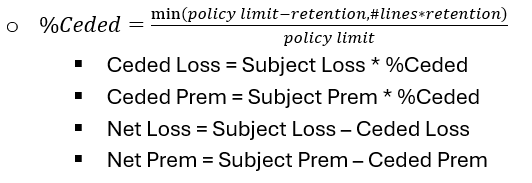
FRIEDLAND (REINSURANCE) - EXCESS PER RISK - ALAE IS HANDLED IN ONE OF THREE WAYS

• Included with loss before calculating excess of loss coverage

• Included pro-rata

• Not included

FRIEDLAND (REINSURANCE) - ULTIMATE LOSS WITH CAT ADJUSTMENT

• Step 1: by treaty year, subtract out REPORTED large CAT losses from CAT losses

• Step 2: develop CAT losses using a CDF and add in the ESTIMATED ULTIMATE of the large CAT losses afterwards

• Keep in mind

  • For a reinsurer covering catastrophe losses, the large catastrophe losses are included in the development triangle for property catastrophe losses when calculating LDFs.

  • The timing within a year of large loss events can also distort loss triangles

  • The actuary can get estimates of ultimate losses for large catastrophes from the claims team and from catastrophe models.

FRIEDLAND (REINSURANCE) - CURRENCY EXCHANGE RATE CHANGES

Use the prevailing exchange rate (latest diagonal) to convert currencies; avoiding distortion

CLARK - PROCESS VARIENCE

VARIANCE DUE TO RANDOMNESS OF THE INSURANCE PROCESS

• Loss model assumptions

  • Assume incremental losses have a constant variance/mean ratio, 2

  • Assume incremental losses follow an ODP (over-dispersed Poisson) model

CLARK - PARAMETER VARIANCE

VARIANCE IN THE ESTIMATE OF THE PARAMETERS

• Calculated based on the Rao-Cramer lower-bound approximation, using the second derivative information matrix

  • The info matrix is used to calculate the covariance matrix

  • The actual calculation of the parameter variance is too complex for the exam

CLARK - DISCOUNTED RESERVES

• CV of discounted reserves < CV of undiscounted reserves

  • Because the tail payout has the greatest parameter variance, but is discounted the most

CLARK - KEY MODEL ASSUMPTIONS

• Incremental losses are iid

  • Independent – one period doesn’t impact surrounding periods (this fails if there are calendar year effects such as inflation)

  • Identically distributed – assume the same emergence pattern for all AYs

• Variance/Mean Scale Parameter, 2, is fixed and known

• Variance estimates use approximation to the Rao-Cramer lower bound

CLARK - LDF METHOD

CLARK - LDF METHOD - GRAPHICAL TESTS

• Residuals should be random around zero & have constant variance to assume the growth curve is appropriate

• Examples of graphs:

  • Incremental age 

  • Expected Loss in Each Increment Age

  • Calendar year

CLARK - CAPE COD METHOD

CLARK - CAPE COD METHOD - PREMIUM MUST BE ON-LEVELED SO THAT WE CAN ASSUME A CONSTANT ELR ACROSS ALL AYs

CLARK - CAPE COD METHOD - COMPARED TO THE LDF METHOD

Cape Cod has lower parameter variance because there are fewer parameters to estimate and it uses more information (on-level premium)

CLARK - TRUNCATION POINT MAKES IT SO

WE DON’T EXTRAPOLATE TOO MUCH INTO THE TAIL OF THE G(X) DISTRIBUTION

CLARK - NORMALIZED RESIDUALS

CLARK - NORMALIZED RESIDUAL GRAPHS

FOR ALL GRAPHS, RESIDUALS SHOULD BE AROUND ZERO WITH NO PATTERNS OR AUTOCORRELATIONS

• Normalized Residuals vs Increment Age

  • Tests how well loss emergence curve fits incremental losses at different development periods. 

    • See whether the curve overestimates for some development periods and underestimate for others

• Normalized Residuals vs Expected incremental loss

  • Check if variance/mean scale parameter is constant. 

    • If not constant, see residual clusterd closer to zero at either high or low expected incremental losses

    • If so this assumption may not be appropriate

• Normalized Residuals vs Calendar year

  • Test for diagonal effects. 

    • High/low residuals for a specific calendar year might be evidence of calendar year effects

CLARK - VARIANCE OF PROSPECTIVE LOSSES

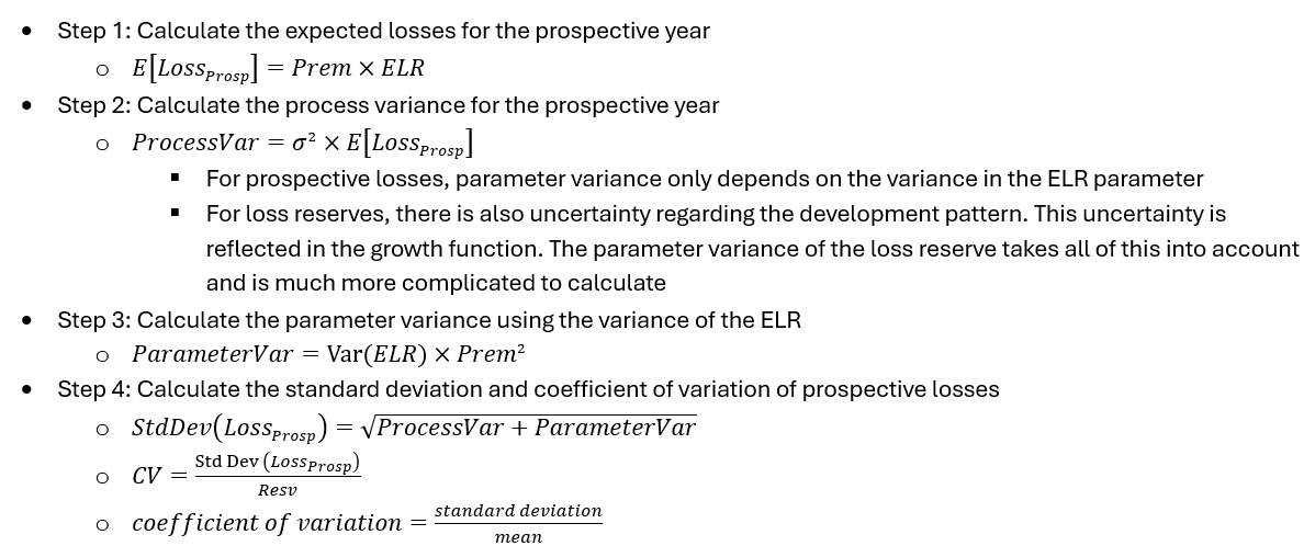
CLARK - VARIANCE OF CY DEVELOPMENT ADVANTAGES

THE MODEL CAN BE TESTED IN A RELATIVELY SHORT TIME

CLARK - BEST FIT PARAMETERS MLE - CALCULATE LOG-LIKELIHOOD

CLARK - BEST FIT PARAMTERS MLE - TWIST

DATA PRESENTED IN THOUSANDS! TRANSFORM THE DATA SINCE THIS WILL AFFECT THE MLE TERM

MACK CHAIN LADDER - MACK ASSUMPTIONS

• Expected losses in the next development period are proportional to losses-to-date

  • The same LDF is used for each AY

  • Uses most recent losses-to-date to project losses, ignoring losses as of earlier dev periods

  • Test: linear relationship between Loss_k+1 & Loss_k through the origin (no intercept)

• Losses are independent between accident years

  • Use the calendar-year test to see if there are calendar year effects such as changes in claims handling

• Variance of losses in the next development period is proportional to losses-to-date by a factor that varies by age

  • Plot the residual graph with this assumption 🡪 should be 

    • random around zero 

    • without trends

MACK CHAIN LADDER - DISADVANTAGE OF MACK METHOD COMPARED TO BOOTSTRAP METHOD

IT DOESN’T TELL US ABOUT THE SHAPE OF THE LOSS RESERVE DISTRIBUTION, ONLY THE MEAN AND STANDARD DEVIATION

MACK CHAIN LADDER - WEAKNESSES OF THE CHAIN LADDER METHOD

• ESTIMATOR OF THE LAST 2 OR 3 LDFs RELY ON VERY FEW OBSERVATIONS

• DOESN’T WORK WELL FOR THE MOST RECENT AY WHERE LOSSES-TO-DATE PROVIDE A VERY UNCERTAIN BASE TO PROJECT ULTIMATE LOSSES

MACK CHAIN LADDER - RESIDUAL TEST (WEIGHTED RESIDUALS)

MACK CHAIN LADDER - CALENDAR YEAR TEST

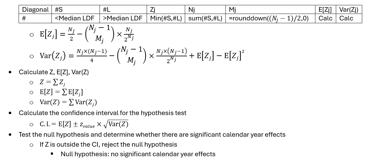
MACK CHAIN LADDER - CALENDAR YEAR EFFECT EXAMPLES

• Major changes in claims handling practices

• Major changes in setting case reserves

• Unexpectedly high (or low) inflation

• Significant changes due to court decisions

MACK CHAIN LADDER - RESERVE CONFIDENCE INTERVAL

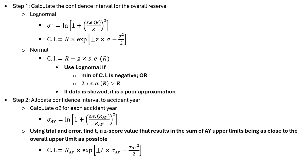
MACK CHAIN LADDER - EMPIRICAL LIMITS

C.I. TOP = CUMULATIVE LOSS * CDF OF MAX (AGE TO AGE FACTORS)

C.I. BOTTOM = CUMULATIVE LOSS * CDF OF MIN (AGE TO AGE FACTORS)

MACK CHAIN LADDER - MSE CALCULATION

MACK CHAIN LADDER - OVERALL RESERVE MSE - IMPORTANT CONCEPT

• MSE of the total reserve > sum of MSE from individual AYs

  • Because the same LDFs are used for all AYs, the loss reserve estimates are positively correlated between AYs, increasing the total MSE

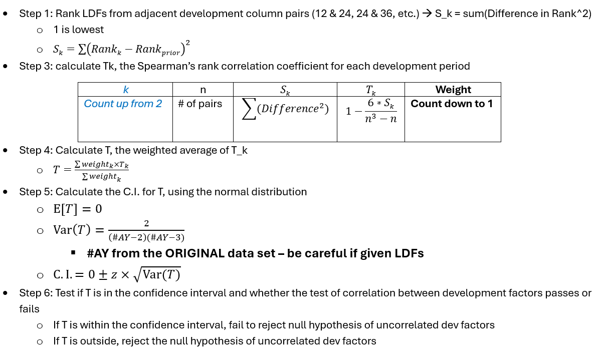
MACK CHAIN LADDER - CORRELATION ADJACENT LDFs (SPEARMAN’S RISK)

• The correlation of adjacent LDFs is a test of Mack’s 1^st assumption that losses in the next development period are proportional to losses-to-date

• Mack Correlation of Adjacent LDFs test looks at the triangle as a whole, not at each column-pair

  • It’s more important to know if correlation between LDFs prevails throughout the triangle

VENTER FACTORS - 6 TESTABLE IMPLICATIONS OF THE MACK ASSUMPTIONS: IF ANY FAIL THEN MACK DOESN’T HOLD UP

VENTER FACTORS - 1. SIGNIFICANCE OF DEVELOPMENT FACTORS (ASSUMPTION 1)

VENTER FACTORS - 2. SUPERIRORITY TO ALTERNATIVE LOSS EMERGENCE (ASSUMPTION 1)

GOODNESS OF FIT TEST: USE ADJ SSE, AIC, BIC (LOWER FIGURES ARE BETTER)

LEAST SQUARES: IF THE CONSTANT IS SIGNIFICANT, THE EMERGENCE PATTERN IS MORE STRONGLY SUPPORTED THAN CL

PARAMETERIZED BF: INCREMENTAL LOSS = f(d)*h(w)

CAPE COD: REQUIRES STABLE LEVEL OF LOSS EXPOSURE

ADDITIVE CL PRODUCES SAME RESULTS AS CAPE COD

VENTER FACTORS - 3. LINEARITY OF THE MODEL: RESIDUALS VS LOSS_K (ASSUMPTION 1)

ASSUMPTION 1 ASSUMES INCREMENTAL LOSS EMERGENCE IS LINEARLY PROPORTIONAL TO LOSS-TO-DATE

IF RESIDUALS SHOW A NON-LINEAR PATTERN, THEN INCREMENTAL LOSS EMERGENCE IS A NON-LINEAR FUCNTION OF LOSS-TO-DATE

VENTER FACTORS - 4. STABILITY OF DEVELOPMENT FACTORS: RESIDUALS VS TIME (ASSUMPTION 1)

Plot residuals against time 🡪 a pattern of high/low residuals indicates instability and is evidence against using the same dev factor for all AYs

STATE-SPACE MODEL: Compares the degree of instability of the observations around the current mean to the degree of instability in the mean itself over time. This helps determine whether to use all of the data or a weighted average that favors more recent years

VENTER FACTORS - 5. CORRELATION OF DEVELOPMENT FACTORS (ASSUMPTION 2)

IF THERE IS A SIGNIFICANT CORRELATION BETWEEN DEV FACTORS AT DIFFERENT AGES, THEN THIS IS EVIDENCE AGAINST CL METHODS

VENTER FACTORS - 6. SIGNIFICANTLY HIGH / LOW DIAGONALS (CY EFFECTS) (ASSUMPTION 2)

IF ANY OF THE DUMMY VARIABLE ARE STATISTICALLY SIGNIFICANT, THEN THIS INDICATES CY EFFECTS

VENTER FACTORS - INFLATION MODEL

VENTER FACTORS - CORRELATED DEV FACTORS

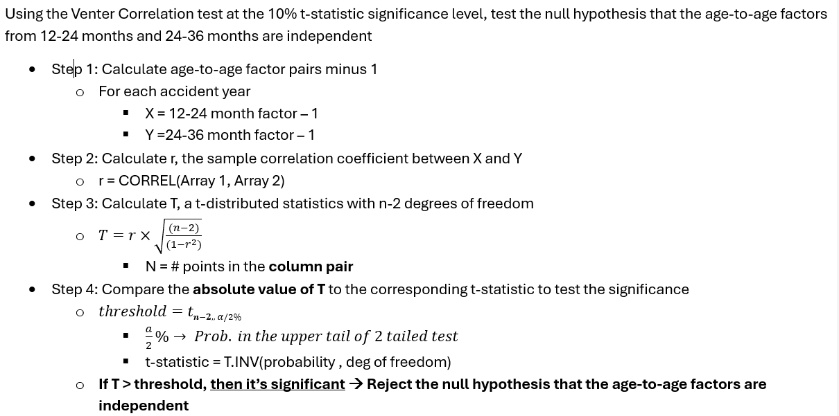
VENTER FACTORS - TESTING FOR CORRELATION IN THE ENTIRE TRIANGLE

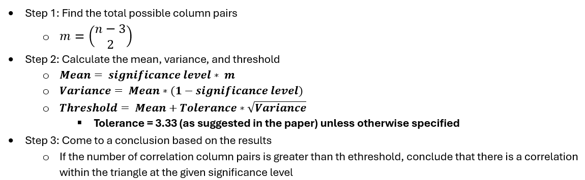
VENTER FACTORS - WHY IS IT IMPORTANT TO TEST CORRELATION IN THE ENTIRE TRIANGLE

VENTER FACTORS - PARAMETERIZED BF - CONSTANT VAIRANCE

VENTER FACTORS - PARAMETERIZED BF: f(d)h(w) - Var f(d)h(w)

VENTER FACTORS - TESTING FOR SIGNIFICANTLY HIGH/LOW DIAGONALS - KEEP IN MIND

IF ABS(COEFFICIENT) > 2 * STD DEV (COEFFICIENT) THEN THE DIAGONAL IS SIGNFICANTLY HIGH (OR LOW)

THIS SUPPORTS THE CL METHOD ASSUMPTION THAT AY’S ARE INDEPENDENT

VENTER FACTORS - GOODNESS OF FIT TEST

VENTER FACTORS - SSE

SUM [(Actual Incremental - Expected Incremental)²]; do not calculate the first dev period

VENTER FACTORS - ADJUSTED SSE

SSE / (N-P)²

N = # OF OBSERVATIONS IN THE SSE TRIANGLE

P = # OF PARAMETERS

Smallest Adjusted SSE is best

Parameterized BF = 2 * (#AY -1)

Chain Ladder = #AY - 1

Cape Cod = #AY -1

VENTER FACTORS - AIC

AIC = SSE * e^(2p/n)

Does not penalize enough for having too many parameters

Smallest AIC is best

VENTER FACTORS - BIC

BIC = SSE * n^(p/n)

Smallest BIC is best

SHAPLAND - GOAL OF BOOTSTRAP MODEL

• create a full distribution of possible loss reserve outcomes, not just a point estimate or the mean and variance like in the Mack approach

  • Do this by sampling residuals from the original loss triangle to create simulated loss triangles, one for each iteration in the simulation

  • Then, an estimated loss reserve is calculated for each iteration

SHAPLAND - BOOTSTRAP DIAGNOSTICS: PURPOSE

• Test model assumptions

• Gauge how well the model fits the data

• Help guide adjustments of model parameters

SHAPLAND - BOOTSTRAP DIAGNOSTICS: RESIDUAL GRAPHS

• residuals should be random around zero for the following graphs

  • Residuals vs CY

  • Residuals vs Dev Period (look for heteroscedasticity)

  • Residuals vs AY

  • Residuals vs Fitted Incremental Loss

SHAPLAND - BOOTSTRAP DIAGNOSTICS: NORMALITY TEST

• Normality Test

  • Normality isn’t required but Shapland mention this as a diagnostic to review

  • If residuals are close to normal you should see

    • Normality plot with residuals in line with the diagonal line

    • High R^2 value and p-value greater than 5%

  • AIC and BIC can be used to compare different models to see which model is closest to Normal while penalizing for extra parameters

SHAPLAND - BOOTSTRAP DIAGNOSTICS: OUTLIERS

• Use a box-whisker plot to identify outliers

• Outliers may simply be extreme but realistic values – in which case they should stay in the data

• Remove the value and treat like a missing value or

• Identify and exclude outliers from the LDF calculation and residual calculations, but re-sample the corresponding incremental loss for the sampled triangles

SHAPLAND - BOOTSTRAP DIAGNOSTICS: PARAMETER ADJUSTMENT

• Look at residual graphs and adjust parameters in the model by adding or removing additional parameters

SHAPLAND - BOOTSTRAP DIAGNOSTICS: MODEL RESULTS

• Standard error 

  • should increase from older to more recent years

  • Total standard error should be larger than the standard error for any individual year

• CoV 

  • should decrease from older to more recent years

  • Total CoV should be less than any individual year

  • CoV could rise in the most recent years due to

    • Parameter uncertainty in most recent years could overpower process uncertainty

    • The model could be overestimating uncertainty

SHAPLAND - MULTIPLE MODELS: MODEL RISK

• risk that the model doesn’t reflect the “true” loss-generating process for future losses. Weighing together multiple reasonable models helps address this

SHAPLAND - GLM SETUP

• Step 1: Calculate incremental loss triangle

• Step 2: Calculate the log-link triangle (natural log of each incremental loss)

• Step 3: Specify the model framework

• Step 4: Model specification (Y=X * A)

• Step 5: Set up the Solution Matrix (Weight Matrix)

• Step 6: Discuss how the α and β parameters are solved for