AP Statistics

Quantitative Variable

Numerical Values

Categorical Values

Names or group labels

2 graphs for categorical variables

• Bar graphs

• Mosaic plot

Quantitative Variable

• Discrete: whole numbers

• Continuous: infinite numbers

Describe Distribution SOCV

• Shape

• Outliers

• Center

• Variation

How to describe the standard deviation

“The context varies by SD from the mean of x”

Mean and SD and greatly (blank) while the median is (blank)

• affected by outliers

• not

For symmetric use (blank) and skewed and outliers use (blank)

• mean, SD

• median

IQR method

• low outlier < Q1 - 1.5IQR

• high outlier > Q3 + 1.5IQR

The (blank) percentile is the value that p% of the data (blank)

• pth

• less than or equal to it

Q1 Percentile

Median Percentile

Q3 Percentile

• 25th

• 50th

• 75th

Standardizing a distribution explanation/z score

“context is when the z score standard deviations above/below mean”

What happens to the shape if you add/subtract/multiply/divide by a value?

it stays the same.

When happens to the center when you add/subtract/multiply/divide

it changes according to the value

What happens to the variability when you multiply/divide

it changes according to the value

Standardizing a distribution means the mean and standard deviation is

0 and 1

Skewed right

symmetric

Skewed left

• mean > median

• mean = median

• mean < median

Empirical Rule

68, 95, 99.7

How to find proportion

NormalCdf

When given proportion

InvNorm

Explanatory

Response

• x variable

• y variable

Describe a relationship DUFS

• Direction

• Unusual behavior

• Form

• Shape

+Context

How to describe correlation

“The linear relationship between x and y is (strength) and (direction)”

Coefficient of Determination r² context

“The percent of the variation in y explained by the linear relationship with x”

Z-Score formula

value-mean/SD

Residual formula

Actual-Predicted

Residual Context

“The actual context was residual above/below the predicted value for x = #”

Interpretations

“when x=0 context, the predicted y context is y-int.”

“for each additional x-context, the predicted y context increases/decreases by slope.”

What is good residual plot and what is bad one?

• Good = no pattern

• Bad = pattern

High Leverage

Influential

• Very large x values

• if removed, the slope changes, y intercept and r

What is wrong with convenience sampling and voluntary sampling?

Leads to bias

Simple Random procedure

1. Label Individuals

2. Randomize (number generator, names in hat)

3. Select

Stratified Random Sampling

• Splits the population into groups with like-characteristics (strata)

• Chooses randomly from each Strata

+low bias and low variability

Cluster Random Sampling

a sample from some of all the groups

Different types of Bias

• Undercoverage

• Nonresponse

• Response Bias

A confounding variable affects the (blank)

• response variable

• also related to the explanatory variable

Experimental Units

What/who the treatment is used on

Treatments

What is done or not done to the experimental units

How to make a well-designed experiment

1. Comparison

2. Random Assignment

3. Replication

4. Control

How to make a block design

Separate subjects into blocks and then randomly assign treatments

Matched Pair Design

1. Subjects are paired and then randomly assigned to a treatment

2. each subject receives two treatments (order of treatment is randomized)

What is Statistically significant

When results of an experiences is unlikely (less than 5%) to happen purely by chance

if significant we evidence that the treatment caused the difference

A random sample allows us to (blank) our conclusions to the population from which we sampled

generalize

Random Assignment allows us to conclude (blank) in the response variable

a treatment causes change

Long run relative frequency

• always between 1 and 0

• short run unpredictable

• long run is predictable

Law of Large Numbers

Simulated probabilities tend to get closer to the true probability as the number of trials increase

Simulation

a way to model random events, such that simulated outcomes closely match real world outcomes

Evidence for a claim

• Assuming a claim is true, find the probability of getting the observed result or more extreme

• <5% statistically significant evidence against the claim

P(E) List all possible outcomes

number of outcomes in E/total outcomes in sample space

Complement rule

• P(A^c) = 1 - P(A)

• probability of the event not happening

P(A and B) / P(A∩B)

both events will occur

P(A or B) / P(A∪B)

one or the other or both

Addition rule when P(A or B)

P(A) + P(B) - P(A and B)

P(A/B) given probability

P(A and B) / P(B)

Independent events

• One event does not change the probability for another

• P(A) = P(A/B) = P(A/B^c)

General Multiplication Rule

P(A and B) = P(A) x P(B/A)

General Multiplication Rule when variables are independent

P(B/A) = P(B) so P(A and B) = P(A) x P(B)

at least 1 probability

P(at least 1) = 1 - P(none)

Combining Random variables

• mean + mean

• mean - mean

• √SD²+SD²

Binomial Random Variable requirements

• Binary

• Independent

• Number of trials

• Same Probability

P(x=k)

binompdf

P(x<k)

binomcdf

Mean and Standard deviation for binomials

M = np

SD = √np(1-p)

10% condition

For a random sample without replacement the size of the population has to be n<0.10

Geometric distribution requirements

• Binary

• Independent

• Trials until success

• Same probability of success

Mean and Standard Deviation and Shape of Geometric distribution

• M = 1/p

• SD √1-p / p (ONLY TOP PART)

• skewed right

A statistic is used to (blank)

estimate a parameter

Sampling Distribution Definition

The distribution of values for a statistic for all possible samples of a given size from a given population

Biased Estimator

overestimates or underestimates the true population parameter

Unbiased Estimator

mean of the sampling distribution is equal to the population parameter

A good statistic has a (blank) and a (blank)

• low bias

• low variability

Steps to check the Sampling Distribution of p hat

• Z score as well

Shape Normal: np>10 and n(1-p)>10

Center: M=p

Variability: √p(1-p)/n

P hat - p / √p(1-p)/n

How to check sampling distribution x hat

Normal if distribution is normal

M = M

SD = SD/√n

Central Limit Theory

The sampling distribution of x hat is approximately normal when the sample size is large enough (n>30)

Confidence Interval

point estimate +- margin of error

interval (A,B)

P.E A+B/2

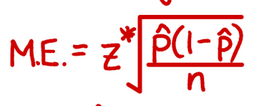
M.E B-A/2

How to interpret the Confidence interval

“We are % confident that the interval from A to B captures the true context.”

All values from A to B are plausible

How to interpret the Confidence level

“If we take many, many samples and calculate a confidence interval for each, about % of them will capture the true context.”

When you increase C.I and M.E

wider interval

increase trials and lower M.E

narrower interval

Conditions for C.I for proportion

1. Random Sample

2. 10% condition n < 10

3. Large Counts np>10 and n(1-p)>10

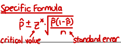
Specific Formula for C.I for proportion

The 4 Cs for Proportion inference

1. Choose procedure, parameter, confidence level

2. Check Conditions

3. Calculate

4. Conclude interpret

Choosing a Sample Size

also when p is unknown, use 0.5 and if n is a decimal you round up

How to evaluate a claim

(+,+) convincing evidence 1st proportion is greater

(-,-) convincing evidence that 1st proportion is less

(-,+) no convincing evidence of a difference

Null Hypothesis and Alternative

H_0: p = null value

H_a: p < null value, p > null value, p ≠ null value

How interpret p-value

• Assuming the null hypothesis is true, there is a p value probability of getting p hat of (blank) or more extreme purely by chance

• Because p-value is < 0.05 we reject H_o and we do have convincing evidence for H_a context

• Because p-value is > 0.05 we reject H_a and we do not have convincing evidence for H_a context

Calculate test statistic for Parameter

test statistic = statistic - parameter / SD

p value for a 2 sided parameter

p value = area x 2

Type I error

Null is true but we reject it

Type II error

Alternate is true but fail to reject Null

P(type I error)

P(type II error)

Type I = 0.05

Type II = 1 - power

Power Equation

P(reject Null/Accept alternative)

Interpret Power

“If the alternate is true (specific value in context) there is a power probability of finding

Conditions for constructing C.I for mean

1. Random Sample

2. 10% condition

3. Normal Sample n>30 also if the distribution just looks normla

Degrees of Freedom

n-1

If null Hypothesis is in the interval

Fail to reject Null Hypothesis

If a mean sample is paired that is just (blank)

a one sample test, not two sample

x² is the (blank)

goodness of fit

Null Hypothesis and alternate for chi square

• The claimed distribution of categorical variable is true

• The claimed distribution of categorical variable is not true

Test statistic and p-value for chi squared

(O-E)²/E

Expected = np

df = # of catergories - 1

x²cdf(x²,9999,df)