FiWi

Meyer (1990)

aim to quantify the sufficient statistics of the Baily Chetty formula (specifically the moral hazard parameter) using DiD

potential problems with randomized experiments

• external valididity

• attrition bias

• hawthorne effect (people behave differently because they know that they are part of an experiment)

• contamination bias (subjects in control groups may also receive some kind of treatment)

• substitution bias (control group may seek substitutions for treatment)

• general equilibrium effects (can it be scaled up?)

Krueger (1999)

example of a large randomized experiment, measure the effect of class size on educational attainment

randomize within schools (assign kids to dif. kinds of classes)

find that small classes better educational attainment but don’t in classrooms with aides

Card and Kruger (1994)

DiD example paper, study the effect of a minimum wage increase in new jersey

Setting; New Jersey raises state level minimum wage from 4.25$ to 5.05$, while PA leaves it at 4.25

Finding: no detectable effect of minimum wage increase on employment

Angrist and Krueger (1991)

IV example paper, use quarter of birth as an IV for years of schooling

find a negative effect on years of education when born in an earlier quartal; find a positive effect of years of education on future earnings in 2SLS

Lee (2008)

RD example paper; estimate the “incumbent effect” i.e. the effect of a person holding a political office on their probabilitz of winning the next election.

Compare candidates who won by a very close margin in the last election, to those who lost by a very close margin, and their outcome in THIS election as an outcome. The running variable is the vote share in the last election

Clay and Greenstone (1995)

attempt to measure externalities using a market-based approach.

typically no market for an externality exists, but we can elicit externality validation if there is a market indirectly linked ot the externality.

Clay and Greenstone use house prices as a reflection of peoples’ utility from living in a local area, aka a capitalization approach

they study the effect of air pollution, with the Clean Air Act as a natural experiment.

• Counties that had high air pollution before the policy went into effect were treated, as they were required to come down below the pollution level ceiling

• Counties with low pollution don’t have to reduce all that much

Use DID comparing treated vs control counties over time.

Result: a 1% decrease in pollution causes about a 0.25% increase in house prices.

Doyle and Samphantharak (2008)

Question: to what extent are petrol taxes passed through to consumers?

Strategy: DiD using state-level changes to petrol taxes in the U.S.

Petrol price spike in 2000 triggered tax relief programs in some states

• Indiana suspends petrol tax in July, reeinstates in Oct.

• Illinois suspends in July, reeinstates end of Dec.

• Neighboring states as control group

They find that when the tax is removed, consumer prices fall significantly. Likewise, when the tax is reinstated, consumer prices also jump back up. Takeaway: consumer incidence on petrol tax is high (likely due to consumers having fairly inelastic demand for petrol)

Hastings and Washington (2010)

Question: how do welfare transfers affect grocery store pricing (question of policy incidence)

Setting: US “food stamps” where low-income households receive vouchers for food (nevada)

Their strategy is to use the timing of transfers (food stamps always given out at the first of the month) and then compare how prices change over the course of the month in high poverty (foodstamps common) areas, and low-poverty areas.

Main result: prices increase at the beginning of the month in high-povery areas → the transfer has some effect on producer surplus

Note: the regression includes week of the month dummies with a dropped first week dummy. therefore, later treat x week dummies have a negative effect because prices are LOWER then than in the base week.

Acemoglu & Angrist (2001)

Question: can mandated workplace benefits hurt workers?

positive analysis

examines the effect of the design of specific policies

tax neutrality

[taxation of a good] economic incidence is independent of statutory incidence

what is the main factor in estimating the efficiency cost of tax-transfer schemes?

labor supply responses

dimensions of labor supply responses

• quantitative dimensions

  • hours workerd for those who are working (intensive margin)

  • labor force participation (extensive margin)

• qualitative dimensions

  • effort on the job

  • type of job (occupation, industry, etc)

  • education

  • location and migration

Eissa (1995)

Use the Tax Reform Act of 1986 (TRA86) as a natural experiment in income tax rates. The reform cut marginal tax rates at the top more than further down in the distribution.

Income taxation is joint in the USA - taxation rate depends on husband’s income

DiD with women whose husbands’ income was in the 99th percentile being treated, and wives with husbands’ income in 75th/90th percentile being control.

Examine the effect on the labor participation rate (extensive), as well as effect on hours worked, conditional on labor market participation (intensive).

Main findings: participation elasticity of 0.5, hours-worked elasticitity of 0.4, total elasticity 0.9. Despite being large, many of these effects are not significant.

Study suffers from paralllel trends problems: upward trend in the female labor supply during that time, and moreso among 99th percentile women as they start from a lower baseline; alos: changes in marriage patterns over time, with a trend towards “assortative mating” - the women marrying these high income men are themselves likely gifted in some manner - also hurts CTA.

Cesarini et al. (2017)

Study the labor supply effects of winning the lottery, which corresponds to a pure income effect (which is, by the way, difficult to measure independently)

Setting: Sweden, administrative data linking wins in lottery to labor market behavior.

Find an implied income effect of around -0.1, with smaller effects on the spouses of winners (implies household coordination in labor supply)

Tazhitdinova (2022)

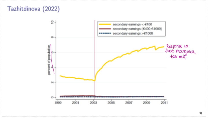
Study the 2003 tax reform in Germany, which made mini-jobs with earnings under 400 euros tax free (including secondary jobs)

• this amounts to a marginal tax cut of 20-60%, depending on couples’ joint earnings

• close to pure substitution effect, because it only changed the tax rate on a small amount of income, no real change to voerall net income.

find sharp increase in the share of population holding a secondary job, and no offsetting effect on primary earnings, meaning an overall INCREASE in labor supply

characteristics of mini-job workers: women, foreign-born, low-educated, low primary earnings

Rationales for Social Insurance

1. Market failure in private markets due to asymmetric information or adverse selection

2. Individual failures, e.g. myopia, self-control problems, lack of information

3. Equity concern: even if the private markets work, individuals with higher risk will have to pay more; may not want this from an equity perspective (considered unfair, especially if the differences in risk are due to “endowments”)

4. Administrative costs: may be more efficient to have a single public insurance compared to many private insurers

Saez, Slemrod, and Glertz (2009)

Attempt to estimate the elasticity of taxable income using a top income share approach.

Basic (non-specific) ETI estimator: [log(s₁) - log(s₂)]/[log(1-t₁)- log(1-t₂)]

where s_1,2 are share of income in the top income bracket in periods 1 and 2, and t_1,2 are the marginal tax rates on the top income bracket in periods 1 and 2.

Results:

• Find that the top income share for the 1% starts increasing in 1981, exactly when the top MTR starts declining.

• There is a sharp jump in the top income share in 1986-1989 which corresponds to the drop in the MTR due to Reagan reforms

• Top income share for top 1% continues to rise in the 1990s despite increases in the MTR

• The next 9%’s income share in the income distribution display NO correlation with the 1% MTR - implies causality

• ETI seems to be heterogenous across groups/time periods, other confounding trends may also be important

Feldstein (1995)

Studies the Reagan Tax Reform (TRA86) as a natural experiment to determine ETI using a dif. in dif. approach

• TRA18 reduced the top MTR from 50% to 28%, with only smaller tax cuts for lower income groups

• ETI = [Δln(z^T) - Δln(z^C)]/[Δln(1-T^T) - Δln(1-T^C)]

results:

• Taxable income increased by 65.4% compared to medium earners, 50.6% compared to high earners

• Implied elasticity of 2.14 (3.05) when taking high (medium) earners as comparison group

issues with the approach

• Mean reversion problem

• small sample

• does not capture longterm responses

Grueber and Saez (2002)

attempt to estimate the ETI. Use panel data from 1979 to 1990. regress changes in taxable income on changes in MTR.

Δln(z_it) = ε x Δln(1-T_it) + x’_itγ * v_it

remaining issues: results very sensitive to specification, in particular, how to control for non-tax related inequality trends and mean reversion

Find an ETI of around 0.4

Kleven and Schulz (2014)

Use cleaner, “better” data from the entire Danish population over 25 years, with a series of tax reforms creating large vairation

key advantage: the Dnaish income distribution is much more constant over time than the American one

Use a similar method to Grueber and Saez (2002) where they instrument changes to the MTR.

Find an ETI of 0.2 for labor income.

The Four Types of Moral Hazard

1. Reduced precaution against entering the adverse state

2. Increased propensity of claiming the adverse state (f.e. disability)

3. Increased expenditure when in the adverse state (f.e. healthcare)

4. Supplier responses to insurance against adverse state

   1. Employer might protect workers from being fired less, if unemployment is not so bad.

What are the main branches of social insurance and what risks do they insure against (also, expenditure size of that branch in SI)

• Unemployment Insurance: nsurance against consumption risk of becoming unemployed (44 billion euros)

• Health insurance: insurance against a large healthcare expenditure (327 billion euros [2nd-largest])

• Old-age pensions: (i) living too long to afford, (ii) not being able to work in old age (400 billion euros [largest])

• Disability Insurance: not being able to work due to disability (included in pensions, 21 billion euros)

• Long-term care insurance: not being able to care for oneself at old age (68 billion euros [third-largest])

• Accident insurance: healthcare expenditure/lost earnings due to a work accident (16 billion euros)

Deductibles, Copayments, and Coinsurance (definitions)

Deductible: The patient has to pay the first eX of healthcare expenditure

Copayment: The patient has to pay X for each unit of healthcare

Coinsurance: The patient has to pay X% of healthcare expenditure

Grueber (1997) on quantifying consumption drop when entering unemployment

Wants to determine by how much C, in practice, falls when a person enters unemployment.

Uses Panel data methodology. Key identification challenge: benefits an individual actually receives are correlated with their own characteristics/state of residence (endogenous), so Gruber uses a simulated instrumental variables approach — he simulates what UI benefits a hypothetical, fixed sample of people would receive under each U.S. state's rules over 20 years, and uses this simulated benefit level (which varies only with policy rules, not individual behavior) as an instrument for the individual's actual benefit/replacement rate.

uses the following regression:

(C_e -C_u)/C_e = β₁ + β₂(b/w) + X’γ + StateFE + TimeFE + e

β₁ is the drop in consumption without getting any gov support = .23 → consumption drops by 23% when becoming unemployed if you don’t receive any gov support

β₂ is the effect of the replacement rate in easing consumption fall = .28 → the fall in consumption falls by .28 for each unit of replacmeent rate.

This allows us to estimate what the fall in consumption between states that we use in Baily-Chetty is, which is then this β₁ + β₂(b/w) term → from that, back out the ideal b.

what markets have adverse/ advantageous selection, and which have no evidence to claim that?

• adverse selection found: Finkelstein & Poterba (2004) — private pensions/annuities (not accident/health insurance); Einav et al. (2010) — health insurance; Landais et al. (2021) — unemployment insurance

• No correlation between risk and insurance purchase: Cawley & Philipson (1999) — life insurance; Chiappori & Salanié (2000) — car insurance; Seibold et al. (2025) — disability insurance

• Advantageous selection: Finkelstein & McGarry (2006) — long-term care insurance