Epidemiology Methods I Exam #2

When do we conclude that an exposure and an outcome are associated?

If mean/risk/prevalence difference not equal to 0.

If risk/prevalence/odds ratio not equal to 1.

Above holds only in the absence of error.

Error

The extent to which an effect estimate deviates from the truth.

Two sources of error:

systematic error

random error

Systemic error

caused by flaws in the research methodology

Sources:

unmeasured confounders

Measurement error

non-random sampling.

Consequences: bias in the effect estimates.

Random error

caused by chance variations

most important source is sampling variation.

Consequence: lower precision of effect estimates (but no bias)

Sampling variation

The variation in a measure of occurrence or association across random samples from the same source population.

Caused by the at random selection of individuals from the source population.

Random selection and sampling variation

Every individual in the source population has the same probability of being selected for the study participation.

However, in a single study, individuals with certain characteristics may be oversampled by chance.

Random sampling impacts

Causes variation in estimates of ocurence and association.

The estimates vary around the true occurrence or association.

The average estimate across many samples will approximate the true occurence or association.

Standard error

Quantifies the variability in the sampling distribution.

They are used to calculate p-values and confidence intervals for effect estimates.

is a statistical measure that captures the variability in an effect estimate across many hypothetical samples.

Standard error helps us determine the precision of an effect estimate.

Sampling distribution of ratios

Typically right skewed.

Normal sampling distribution

standard error only have a relevant interpretation.

The natural logarithm (Ln) scale for ratios

Range and distribution before transformation: null effect=1

Range and distribution after transformation: null effect=0

Hypothesis testing

The goal of research is determining if there is an exposure-outcome association

Random sampling variation makes it impossible to determine if the hypothesis holds based on the effect estimate only.

Test hypothesis

the value which we compare the observed effect estimate.

Can be any value. but typically we use the null hypothesis.

Null value=0

Risk/prevalence difference

Mean difference

Ln (risk/prevalence ratio)

Ln (odds ratio)

Null value=1

Risk/prevalence ratio

Odds Ratio

P-value

The probability of observing the effect estimate if the test (null) hypothesis is true.

is determined using the test statistic which helps us determine the location of the effect estimate in a normal sampling distribution.

An estimate is statistically different from the test hypothesis if the P-value is <0.05.

Test Statistics

Tells us how many standard deviations the test hypothesis the observed effect estimate is.

Computed using:

-the effect estimate

-the test hypothesis

-the standard error

Statistical significance

Tells us whether there is mathematically meaningful difference in the outcome between the two compared groups.

is not equal to clinical relevance.

Typically a probability of 5% is used as the cut off.

Effect estimates are considered statistically significant when the P-value<0.05.

Alternative hypothesis: there is an association.

Hypothesis testing limitations

It relies on the strong assumption: we can only reject the null hypothesis if the effect estimate is completely unbiased.

P<0.05 does not say anything about the clinical relevance of an effect estimate.

Confidence intervals formula

Confidence interval width

The higher the confidence level, the wider the confidence interval.

Type I error

rejecting the H0 when H0 is true.

falsley concluding there is an association.

If the effect estimate is unbiased then the probability of making a chance finding equals alpha.

Type II error

failing to reject the H0 when Ha is true.

We falsely conclude there is no association.

Happens when the statistical power is too low to detect a statistically significant association (lack of power)

Statistical power depends on:

the sample size

alpha

the size of the true effect

Power

is the probability that we detect an association when in reality there is an association.

1-Type II error

Power Analysis

1. The sample size needed to detect a specific effect size given a specific alpha level and the power level.

2. The minimum effect size that can be detected given a specific level of alpha, power, and sample size.

Clinical relevance

pertains to whether there is clinically/practically meaningful difference in the outcome between the two groups.

-Depends on the size of the effect estimate.

-is context dependent

continuous outcomes: is the mean difference representing a relevant increase/decrease in the outcome.

Binary outcomes: evaluation of the effect size in combination with the background risk; relevant increase/decrease in outcome occurrence.

Statistical significance depends on

The power to detect an effect estimate that is different from the null variable.

Power can be somewhat increased by researchers increasing sample size, increasing alpha.

As power increases more likely to find statistically significant effect estimates.

Implications of statistical significance and clinical relevance

Fundamental problem of casual inference

It is impossible to observe both potential outcomes for the same individual for the same individual over the same time period.

Solution: compare average potential outcomes.

Casual effect

Difference between the ratio of the two average potential outcomes.

Casual assumptions

Exchangeability

Consistency

Positivity

Exchangeability assumption

On average the exposed group and unexposed group are exchangeable in all aspects other than the exposure.

The only characteristic that differs across the two groups is the exposure.

If it holds then we would get the same estimates for E[Y(x)] and E[Y(x*)]

if (hypothetically) we were able to exchange the exposure across the two groups.

Violation of exchangeability

The two differ in aspects other than the exposure and the aspects in which the groups differ also affect the outcome.

Exchangeability and Confounders

Means that there cannot be any unmeasured confounders of the exposure outcome association.

is violated when the distribution of confounders differs across the two exposure groups.

When violated the effect estimate will be biased.

Solutions to the violation of Exchangeability

Randomization

Restriction

Matching

Stratification by confounders

Consistency assumption

The observed outcome for an individual is equal to the potential outcome when the exposure is set to the observed exposure value.

Typically holds in experimental studies where E[Y(x)] and E[Y(x*)] are obtained by randomizing individuals to well defined intervention and control conditions.

Consistency in RCTs

A well defined intervention condition: every person in the intervention condition receives the exact same intervention.

A well defined control condition: every person in the control condition recieves the exact same control.

There is one way in which individuals qualify as exposed/not exposed to vitamin D.

Violations of consistency assumption

The observed outcome for an individual is not equal to the potential outcome when the exposure is set to the observed exposure value.

Violated when two conditions hold.

1. There is various ways in which an individual qualifies as (not) exposed.

2. The exposure association outcome differs across the types of exposure.

Solution to the violations of consistency

Use a more precise definition of the exposure values of interest.

But don’t take too far because definitions come at the cost of generalizability.

Positivity assumption

When defining casual effects based on potential outcomes, we essentially assume that one individual (with all their background characteristics) has a positive probability of taking on both exposure values.

Holds when all probabilities are nonzero.

Violation of Positivity

The probability to observe an exposure level of interest based on a specific combination of confounder values equal to zero.

Solutions to violations in positivity

When one or more probability is zero we cannot make comparisons based on that combination of confounder values.

Solution is to restrict the comparisons to combinations of confounder values for which the probabilities of observing x and x* are both nonzero.

For observing drinking and pregnant women it would be beneficial to restrict the analysis to only women 21 years or older.

Directed Acyclic graphs

DAGs are graphs used to visualize the associations between variables. DAGs are informed by subject matter knowledge regarding the associations among the variables of interest.

DAGs and the Research Process

DAGs can help guide data collection and statistical analyses.

Ideally DAGs are developed at the start of the study

1. Identify confounders that we need to collect data on.

2. Identify mediators that we may want to collect data on.

3. identify potential sources of selection bias.

Basic Features of DAGs

Directed paths- lines with one arrowhead shows that the exposure precedes the outcome and the exposure affects the outcome.

The absence of an arrow conveys that the exposure does not affect the outcome.

Acyclic- none of the paths form a closed loop

Reciprocal effects in DAGs

A reciprocal effect means that the exposure affects the outcome and that the outcome in turn affects the exposure.

Third variables

the two focal variables are exposure and outcome but third variables such as colliders, mediators, and confounders can be present.

Confounder

Affect the exposure and the outcome.

A change in the confounder leads to a change in the exposure and the outcome.

Create an open backdoor path between exposure and outcome.

If we leave backdoor path open then there will be confounding bias.

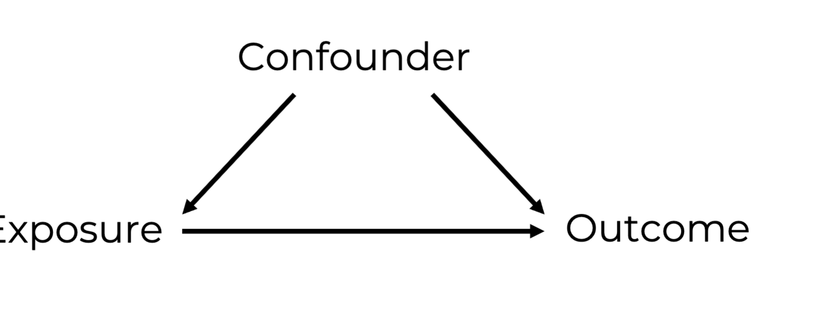
Confounding bias

-The exposure-outcome effect estimates will be larger or smaller than the true size of the exposure-outcome effect.

-The exposure-outcome effect estimate will be nonzero while in truth the exposure-outcome effect is zero.

Mediator

-Affected by the exposure and effects the outcome.

-is on the casual pathway from the exposure to the outcome.

This structure created by a mediator in a DAG is called a “chain”

Changes in the exposure lead to changes in the mediator, and changes in the mediator lead to changes in the outcome. Mechanisms through which the exposure affects the outcome.

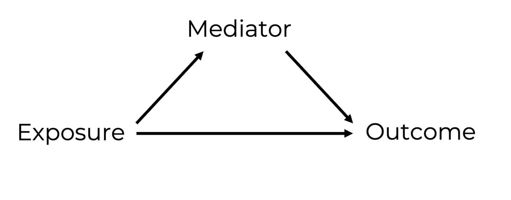
Mediators can be used to decompose

the total exposure outcome effect into

1. An indirect effect through the mediator

2. A direct effect not through the mediator.

Indirect and Direct pathway Mediator

Indirect effect: the effect of the exposure on the outcome through the mediator

Direct effect: the effect of the exposure on the outcome not through the mediator.

Overadjustment bias

In and of themselves mediators do not bias the exposure outcome effect estimate.

When adjusted in statistical analyses mediators cause “overadjustment bias”

After adjustment for a mediator, the exposure-outcome effect estimate represents the direct effect rather than the total effect.

Mediation analysis

A method for estimating direct and indirect effects with corresponding confidence intervals.

It is increasing used in epidemiology to better understand why exposures and outcomes are associated.

Collider

Affected by the exposure and affected by the outcome

is a common cause of the exposure and outcome.

Change in both the exposure and outcome lead to changes in the collider

a consequence of both the exposure and outcome.

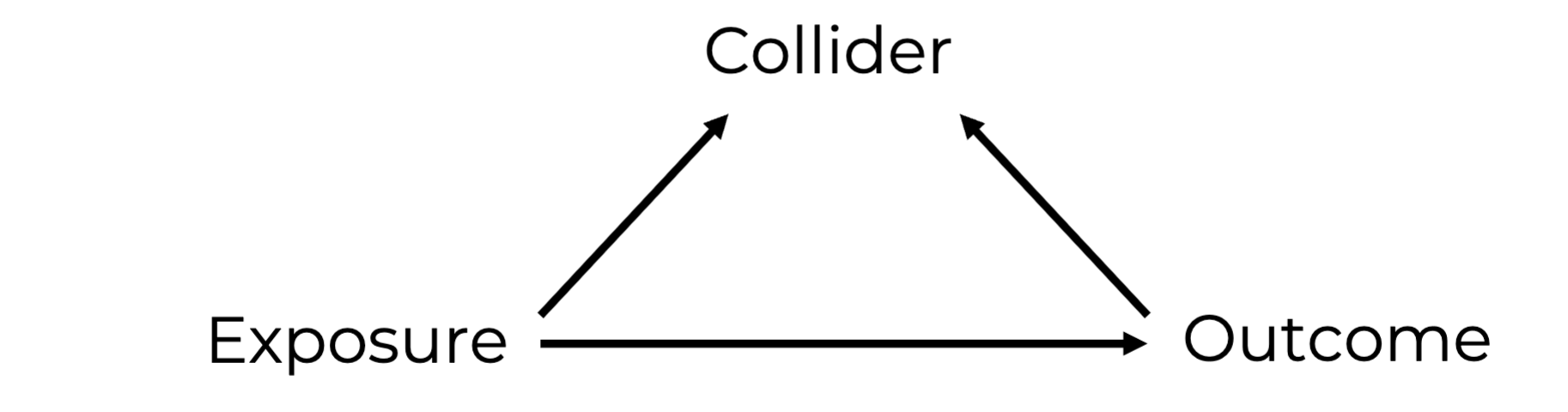
Collider Bias

Colliders do not bias nor explain the exposure-outcome effect.

However colliders can bias the exposure-outcome effect estimates when

1. Selection into the study is restricted to certain collider variables.

2. Adjustment is made for colliders in statistical analyses.

3. Analyses are stratified by the collider.

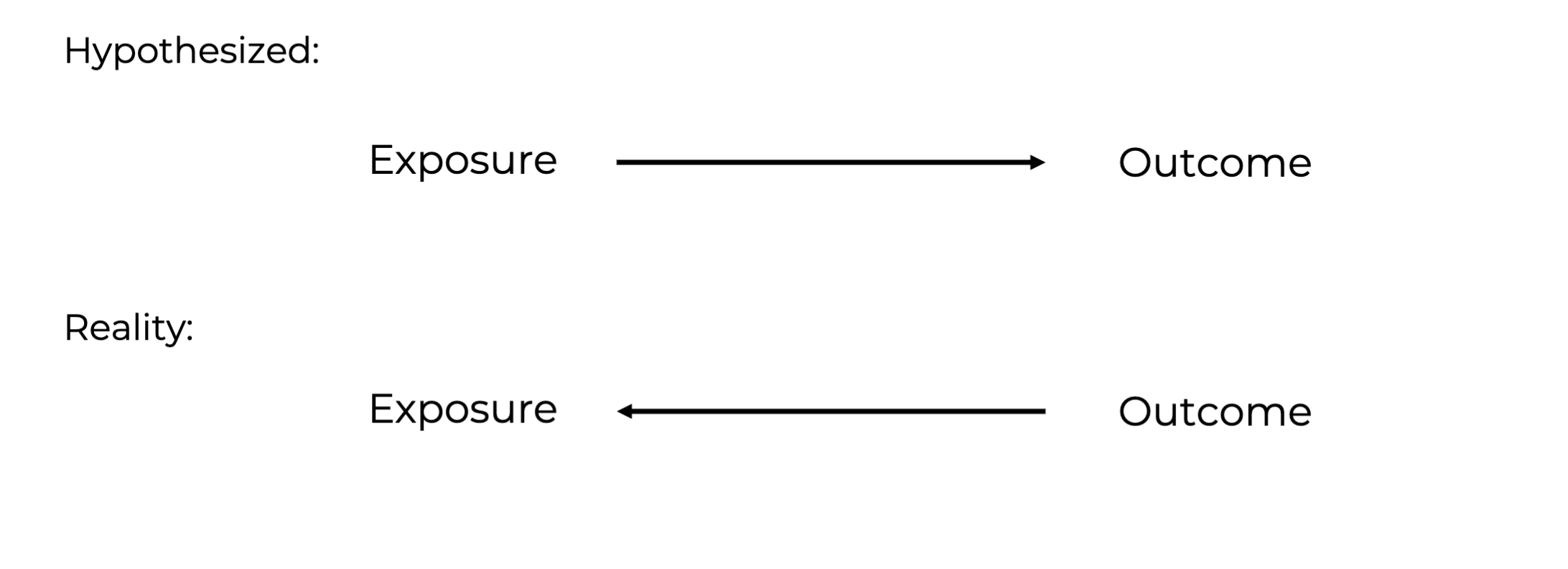
Reverse causation

The hypothesized exposure is in truth consequence of the hypothesized outcome.

can occur in most study designs but cross-sectional study designs are especially prone to reverse causation.

Sufficient cause framework

conceptualizes causation as a collection of multiple causes of outcomes.

A collection of component causes that when all present in one individual causes the outcome in the individual.

Component causes

single causes of outcome.

Rothman’s sufficient component cause model

sufficient cause represents mechanisms that lead to occurence of the outcome.

Causal Pies

Sufficient causes are visualized using pie charts.

Each pie chart represents a sufficient cause and each slice within the pie chart represents a component cause.

Confounding bias is present

The effect estimate will be larger, smaller, of opposite direction, or falsely nonull compared to the true effect.

True exposure-outcome not equal to null value

The exposure outcome estimate will be larger, smaller, or of opposite sign compared to the true exposure outcome effect.

Overestimation due to confounding

When the exposure outcome effect estimate is larger than the true exposure-outcome effect.

Also called bias away from the null.

Occurs when the combined influence of the confounder exposure and confounder effect is the same in direction as the true exposure outcome effect.

Underestimation due to confounding

when exposure outcome effect is smaller than the true exposure outcome effect.

also called bias towards the null

Qualitative confounding

When the exposure outcome effect estimate is in the opposite direction of the true exposure outcome effect.

Nonnull

If the true exposure outcome effect= the null value

Marginal effect estimate

The effect estimate applies to the whole study population.

Conditional effect estimate

The effect estimate applies only to a subset of individuals with specific confounder values.

Design stages to minimize confounding

Randomization

Restriction

Matching

Randomization

Random assignment to the intervention group or control group

The intervention and control group will be exchangeable in all apsects other than the intervention/control condition.

Randomization strengths

Targets both known and unknown confounders because in expectation any factors other than exposure will be equally distributed across the two groups.

Works for confounders on any measurement scale.

Randomization limitations

works in expectation due to sampling variability confounders may still be unequally distributed across groups in any one study.

Protocol violations and drop outs might result in unequal distributions of confounders across the intervention and control group.

It is not ethical to randomize individuals to harmful exposures.

Restriction

Restriction of the study population to one specific level of the confounder.

It eliminates the variation in the confounder, so within the restricted sample it no longer effects the exposure and outcome.

Results in conditional effect estimates.

Restriction strengths

Most effective way to prevent confounding by a known confounder.

Restriction limiations

Does not prevent confounding by unknown confounders.

Reduces generalizability of the findings.

Only works if there is truly no variation in the confounder in the restricted sample.

May not be feasible when there are many confounders and or continuous confounders.

Matching

Compared groups are selected in a way that ensures the same distribution of confounders across groups.

Cohort studies: comparison group is selected in such that the distribution of the confounders matches the exposed group.

Case control studies: controls are selected in such that the distribution of the confounders matches that of the groups of cases.

Types of matching

Pair matching

Frequency matching

Pair matching

One to one individual matching based on potential confounders

For every exposed individual with certain combination of confounder values we include an unexposed individual (or controls) with the same combination of confounder values.

This ensures that distribution of confounder values is the same across exposure groups.

Frequency matching

Selection of groups in such a way that the distribution of confounders is the same across the two groups.

In each exposure group (or cases/controls) a similar proportion of individuals is included with certain confounder values.

Matching strengths

can increase efficiency and power in certain situations.

Matching limitations

Does not prevent confounding by unknown confounder.

May not be feasible and reduce generalizability when there are many confounders and or continuous variable confounders.

one on one matching we may not always be able to find a match.

Limitations of design stage methods to minimize confounding

It is not always feasible to apply design stage methods eg:

The exposure is harmful, so randomization is not possible

Restriction or matching is not feasible because there are too many confounders or continuous confounders.

Randomization or matching failed

Data was not collected with your specific study in mind.

Marginal effect estimate

The effect estimate applies to the whole study population.

Conditional effect estimate

The effect estimate applies only to a subset of individuals with specific confounder values.

Stratification

Perform the analyses separately for different strata of the confounder variable(s).

Results in conditional effect estimates the effect estimate applies only to individuals in that confounder stratum.

Mantel Haenszel methods

Recombine the effect estimates after stratification.

Inverse probability weighting

IPW provides weighted averages of stratum specific effect estimates.

Gives more weight to strata that have a larger number of participants in it.

Individuals are weighted by their inverse of the probability of their exposure value.

Creates a psuedo population in which there are no confounder exposure association.