Final Exam Study

Rank of Matrix

number of linearly independent rows or columns of a matrix

Rank

2

Rank

3

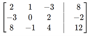
Representing systems of equations as a matrix, what is the augmented matrix

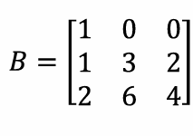
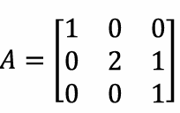
properties of matrix

associative, distributive, tranpose, NOT commutive

Soutions to systems of equations are where they

intersect

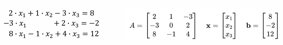
Linear systems can be expressed in matrix form as

[A][x]=[b]

Guassion Elimination solves for

x= inv([A])*[b]

Forward elimination

eliminates variables

Back substitution

solves for variables

Interlopation

estimating intermediate values between data points

Polynamila interpolation

find the polynomial that exactly connects n data points

B spline interpolation

find a piece-wise sum of n basis functions that exactly connects n data points

Linear interpolation a1formula

a1+(a2)x

Quadratic Interpolation formulation

a1+(a2)x+(a3)x²

Higher order polynomial interpolation

a1+(a2)x+..+an(x^n-1)

extrapolation

making a predication not justified by the data

interpolation error decreases

as step size decreases

higher order polynomial interpolation

can lead to high errors

b-spline interpolation approximates

data using sum of simple basis functions

extrapolation can cause

large errors

optimization finds

max or min of f(x), roots of f’(x)

with optimization, there is no gaurantee

to find global min or max

brute force optimzation

tries all values to find max/min

disadvantages of brute force

can miss max/min of points and has huge computational cost

steepest ascent formula

xi+1 = xi+hf’(x)

as x approaches max,

steps get smaller

if h is too small, it will

converge slowly

if h is too big,

it may overshoot maximum

newtons method optimization finds (requires f’’ and may diverge)

local max and min and locations where f’(x)=0

main features of steepest ascent method

max, only needs 1 starting point, must be able to take f’, converges slowly, requires h and may not converge depending on h value

main features of newtons method

max or min, only needs 1 starting point, can diverge, must be able to take f’ and f’’, converges fastest

newtons method vs. steepest ascent

converges faster when near maximum but can diverge

goal of linear regression

to find the line that best fits data

define error or residual formula

ei = yi - fi

coefficient of determination, r²

quantifies % of data explained by the regression line

what does r²=1 suggest about line

100% of data was captured

regression

fitting models to data, usually by minimizing the sum of squared errors

linear regression

has unique solution, coefficients can be calculated algebraically

ways to quantify regression error

SSE and coefficient of determination

linear regression vs interpolation

both involve finding coefficients that best describe the data

least squares approzimation

finds a line that gets as close as possible to the points

matrix in least squares approximation

not square, making exact solution generally not possible

interpolation goes exactly

through all given points

as long as the equations are linear with respect to parameters, linear least-squares can be

reformulated as matrices and be extended to more complex examples wih indp. var or nonlinearities

unlike linear least squares, non linear regression does not guarantee that

a global minimum will be found

brute force non linear approach

manually or programmatically tries all combinaions of parameters

advantages to nonlinear regression

simple to implement, even converge of paramter range

disadvantages to nonlinear regression

computationally costly, on the order of values

goal of nonlinear regression

identify a set of model parameters that is most consistent with experimental data

optimization algorithms are

designed to efficiently search through the possible parameter combinations id identify “best fit” parameter set that minimizes SSE

gradient SSE in nonlinear regression

indicates how much and in which direction the sum of squares error changes as parameter values change

gradient SSE in steepest descent, non linear regression

used to compute direction of steepest slope and parameters are adjusted with step size proportional to the magnitude of it

gradient-based optimization is based on

Levenberg-marquardt algorithm

Levenberg-marquardt algorithm

combines initial steepest asvent algorithm followed by Gauss-newton algorithm to converge to final solution

nonlinear regressions can

preform best fits even when model is nonlinear with respect to parameters

nonlinear regression cannot

guarantee a global minimum, may converge to local minima

optimization methods such as steepest descent or Newton’s method can make

optimization more efficient than brute force

Runge Kutta method

symbol providEues an estimate of the slope of y(x) over the interval from xi to xi+1

Euler’s method local truncation error

measures the error introduced in one step of method assuming that the previous step was exact. As Euler’s method can be obtained through Taylor’s series

Euler’s method local truncation error

O(h²)

Euler’s method global truncation error

is the error at a fixed time, ti, after however many steps the ethod needs to take to reach that time from the initial time O(h)

Euler’s method overview

approximate solution using slope at current size

Euler’s method error depends on

step size

Higher Order Runge Kutta

predict an initial slope k1 and then gradually refine/correct it with other slopes

Midpoint single step error

O(h3)

Midpoint cumultive error

O(h²)

4th Order Runge Kutta Method single step error

O (h^5)

4th Order Runge Kutta Method cumulative error

O(h^4)

Increasing the order of RK increases

the accuracy

Error for RK methods depends on

step size, h

Lorenz Equation - Butterfly Effect

small change in one state of deterministic nonlinear system can result in large differences in later state