Chapter 7: Costs

Explicit costs

direct, out of pocket payments for inputs

Implicit costs

reflect a forgone opportunity rather than an explicit expenditure (opportunity cost)

Opportunity cost

the value of the best alternative use of a resource

Economic costs

implicit costs + explicit costs

What is the opportunity cost if a firm rents capital?

If a firm rents capital, then the rental payment is the opportunity cost

What is the opportunity cost if a firm buys capital?

If a firm buys capital, then the opportunity cost is the amount that the capital could be rented for (e.g., building)

What happens when no rental market exists?

Could use depreciation and forgone interest as opportunity costs

Sunk cost

a past expenditure that cannot be recovered. You IGNORE sunk cost

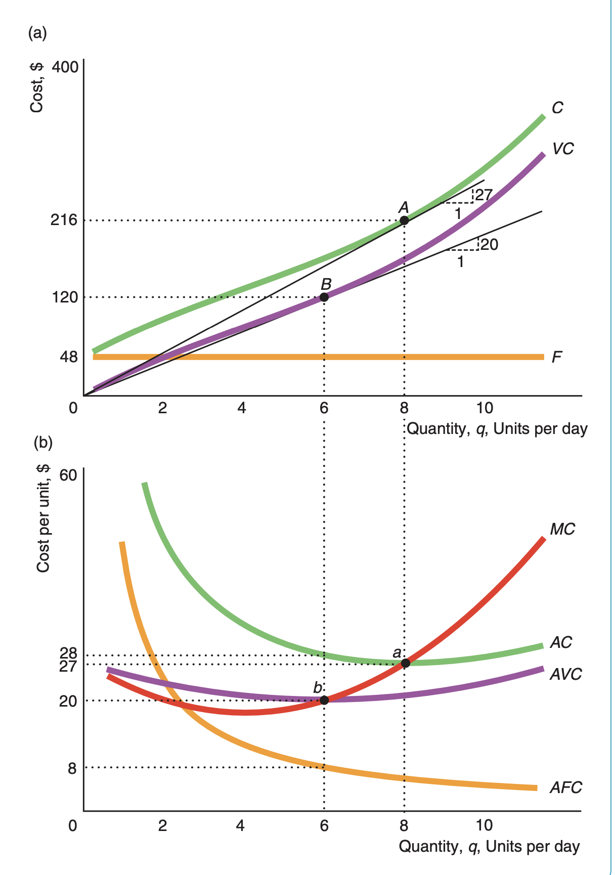
Fixed cost (F)

cost that does not vary with level of output (E.g., land, large machines, rent, insurance)

Variable cost (VC)

cost that changes with output (e.g., labor, materials)

Total cost equation in SR

C = F + VC

Marginal cost (MC)

amount a firm’s cost changes with one more unit of output

MC = dF/dq + dVC/dq

What is MC in short run?

dV/dq

Average cost (AC)

AC = C/q

(or AFC + AVC)

Average variable cost (AVC)

VC/q

Average fixed cost (AFC)

F/q

(*AFC is always falling as Q increases in SR)

What is the relationship between average cost and average variable cost?

AFC = AC - AVC

as q goes up, AC and AVC get closer together

How to calculate variable cost in the short run

VC = wL

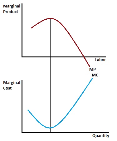
How to calculate change in labor?

MC = w / MPL

The additional output created by every additional unit of labor is

MC = w/MPL

What is the relationship between marginal cost and marginal product of labor?

they move in opposite directions

MC = w/MPL

How does average variable cost change with average product of labor?

AVC = w/APL

AVC and APL move in opposite directions

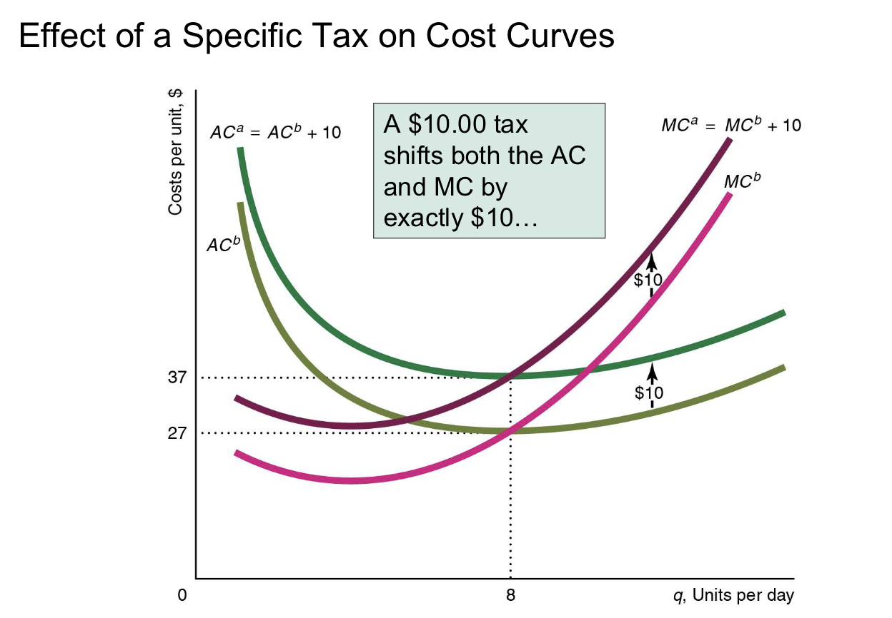
What is the effect of a specific tax on cost?

A specific tax increases VC (not FC). May shift some or all of the MC and AC curves.

In the long-run, fixed costs are ___ rather than___.

in the long-run, fixed costs are avoidable rather than sunk.

T/F: firms can vary both L and K in the long-run so cost of production should be less than in the short-run.

True

Total cost equation in the long-run

C = wL + rK

Isocost line (C)

a plot of all combinations of inputs that require the same (iso) total expenditure (cost)

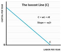
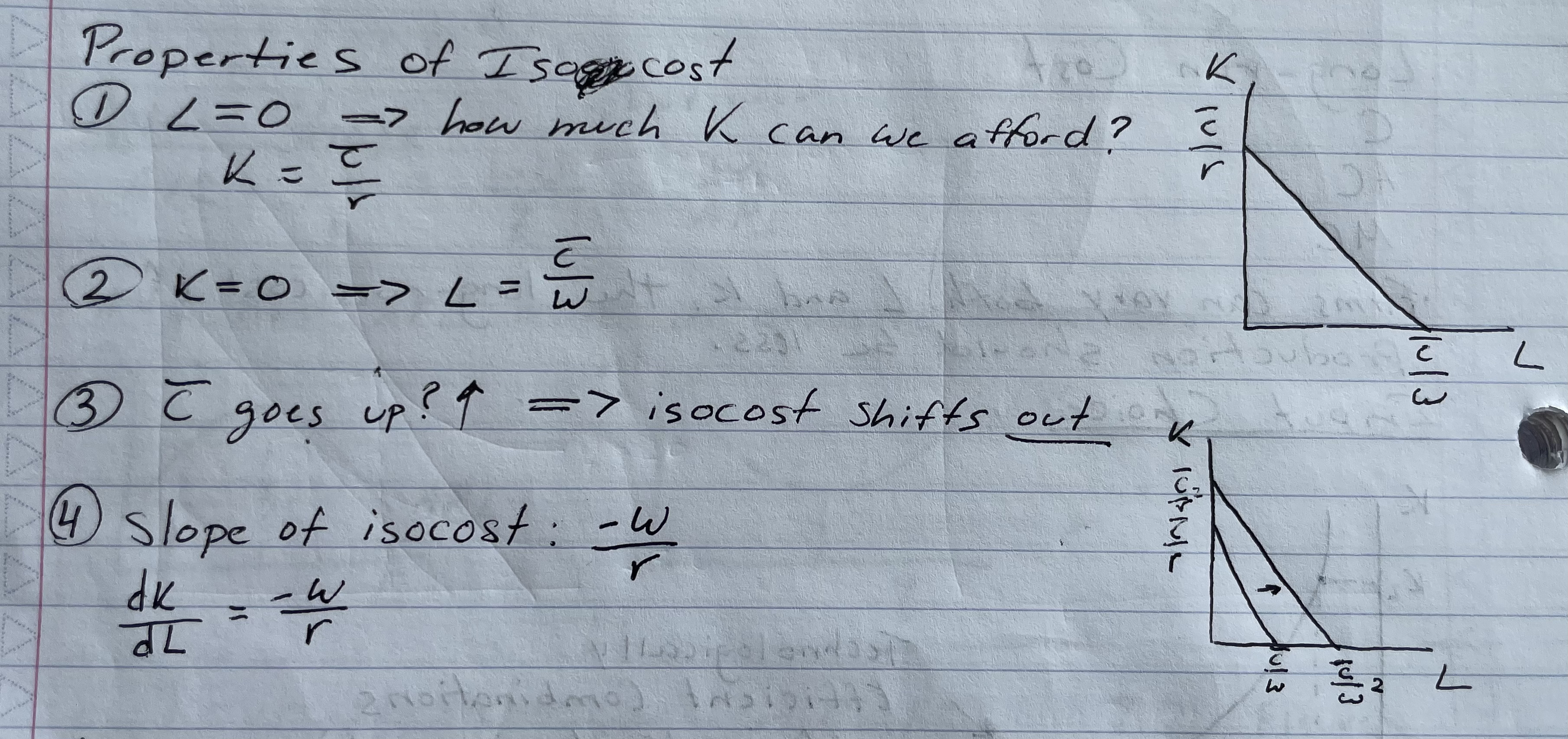
Properties of isocost lines (4)

1. When L = 0, K= C/r

2. When K = 0, L = c/w

3. When C goes up, isocost shifts out

4. Slope = -w/r

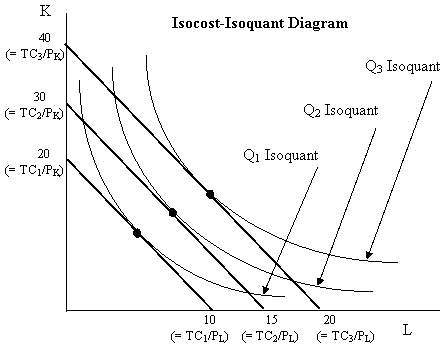
Where is cost minimized on the isocost-isoquant graph?

The point tangent to the isoquant

3 equivalent approaches to find minimum cost in LR

1. Lowest isocost rule (graphical representation)

2. Tangency rule - pick a bundle where isocost is tangent to isoquant.

   MRTS = -w/r

3. Last-dollar-rule

What is the last-dollar-rule?

(pick bundle of inputs where the last dollar spent on one input gives as much extra output as the last dollar spent on any other input.)

MRTS = -MPL/MPK

if MPL/w > MPK/k use labor because last dollar produces more extra output

Steps to find cost-minimizing bundle of L & K using tangency rule (5):

1. Find MRTS

2. Set MRTS = slope of isocost

   MRTS = -w/r

3. Solve for K in terms of L to find long-run expansion path (and plug in w & r here)

4. Solve for L in terms of K

5. Plug 3 and 4 into production function to solve for L and K

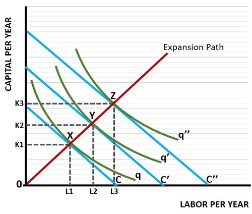
What is the expansion path?

the expansion path goes through the cost-minimizing combinations of inputs for each level of output

(when you solve for K)

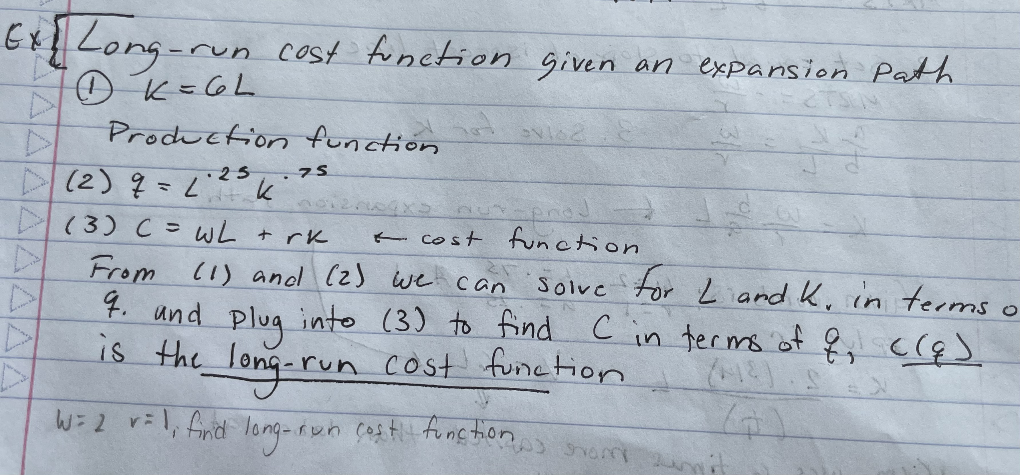
How to find long-run cost function given an expansion path:

You have:

1. K in terms of L (K = 6L)

2. production function

3. LR cost function

   From 1 and 2 we can solve for L and K in terms of q. Plug into 3 to find C in terms of q (C(q)), and that is the long-run cost function.

   

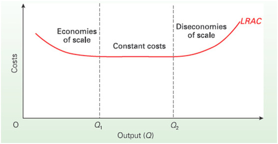
What is the shape of a long-run average cost curve and what does it tell us?

Tells us where economies of scale, constant returns to scale, and diseconomies of scale.

Increasing returns to scale is a sufficient condition of what?

economies of scale

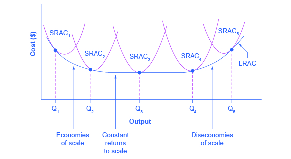
What does a graphical representation look like for a plant of different sizes in the SR & LR?

On the right is economies of scale

On the left is diseconomies of scale

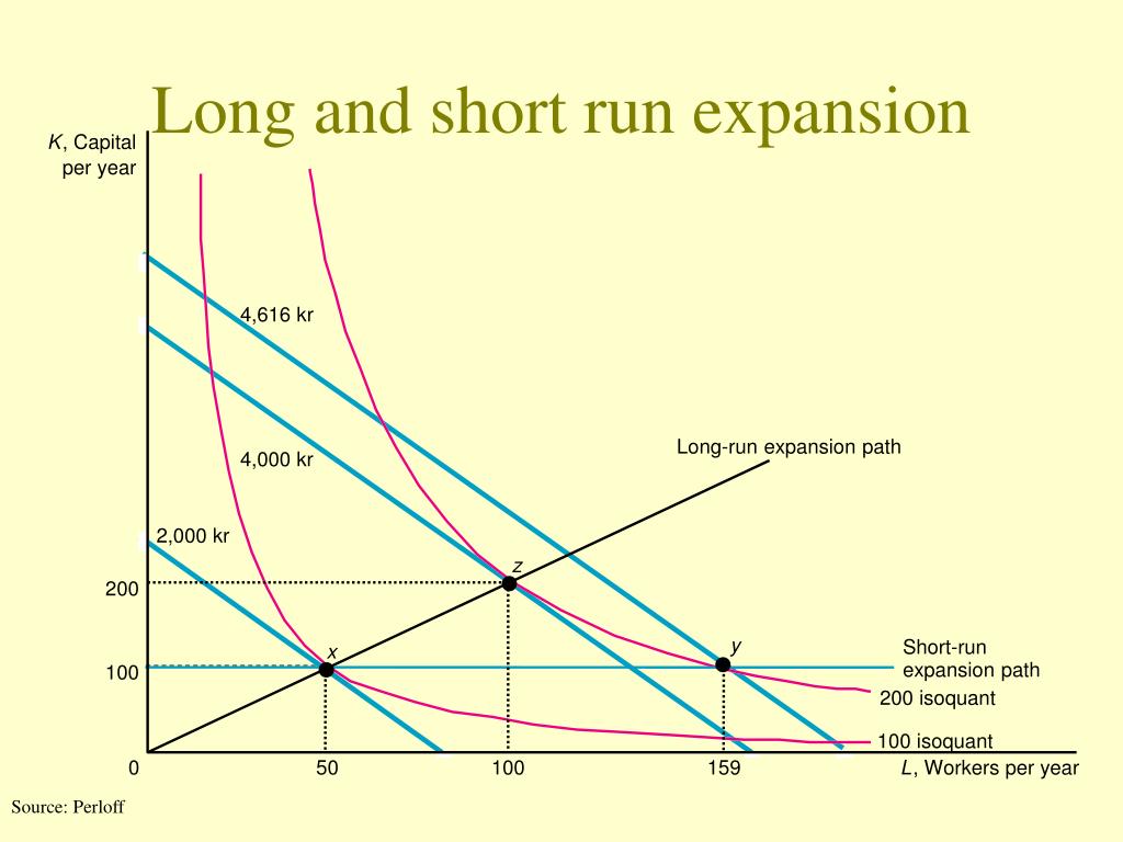
Long-run and short-run expansion paths

short-run expansion path is a horizontal line

(*y has to go on a higher isocost because can only vary labor in the SR)

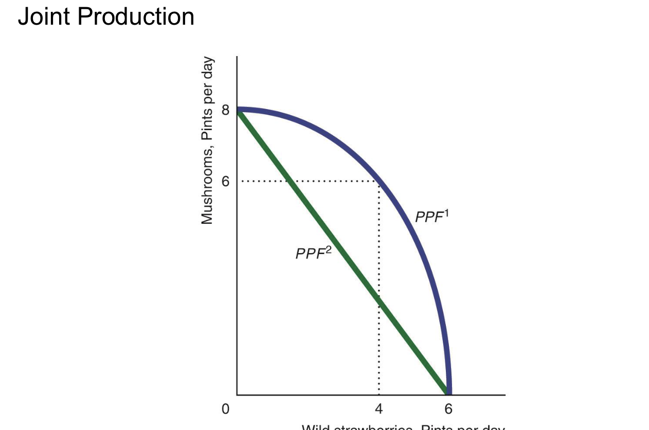
Economies of scope

a situation in which it is less expensive to produce goods jointly than separately (think lumber and sawdust)

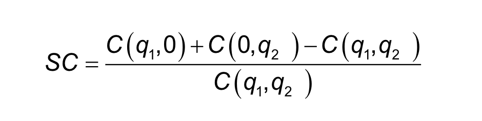
How to calculate scope economies

SC = C(q1, 0) + C(0, q2) - C(q1, q2) / C(q1, q2)

If

SC > 0 → Economies of scope (produce together)

SC < 0 → Diseconomies of scope (produce separately)

What does a PPF tell us about economies of scope?

Concave PPF shows economies of scope

Method to minimize AC

Take the derivative of AC function and set it equal to 0.

(dAC/dq = 0)