AP STATS UNIT ONE

individuals

subjects described by a set of data or part of the set of data

variables

characteristics of individuals

catergorical vs quantitative

categorical variables

places an individual into one of several groups or categories

ex) gender, zip codes, political party, grades

quantitative variables

take numerical values

ex) number of pets, time, height

discrete vs continuous

discrete quantitative variables

countable values

ex) number of siblings

continuous quantitative variables

measurable values

ex) weight

representing categorical data

tables: one way vs two way

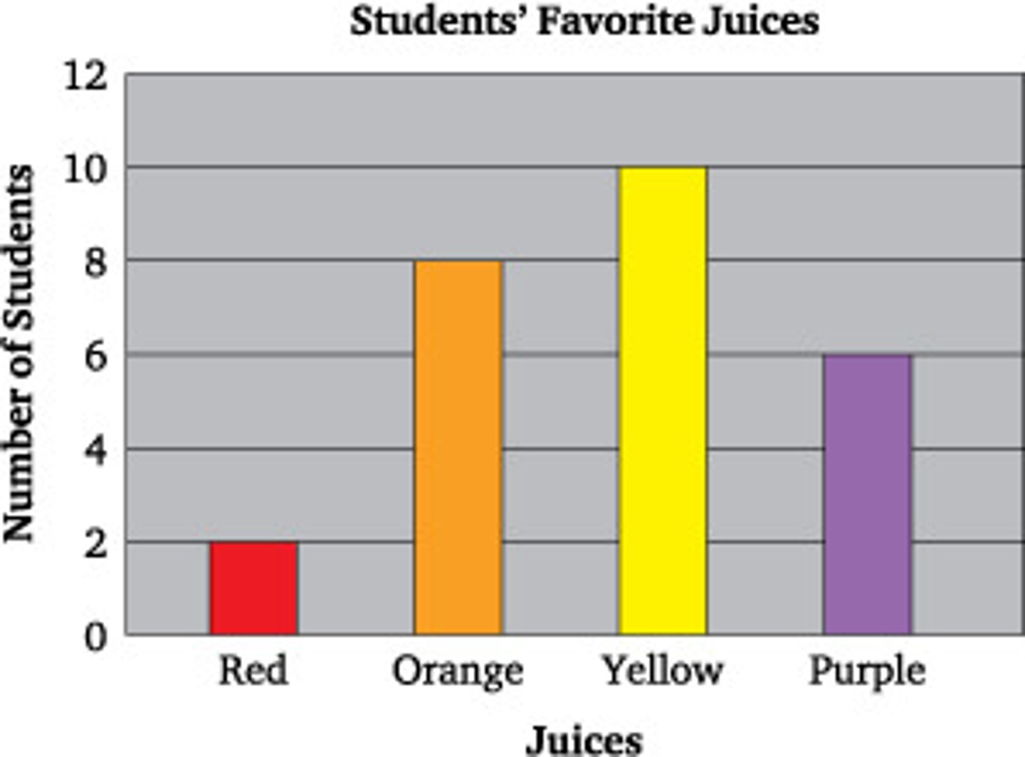
bar graphs

one way table

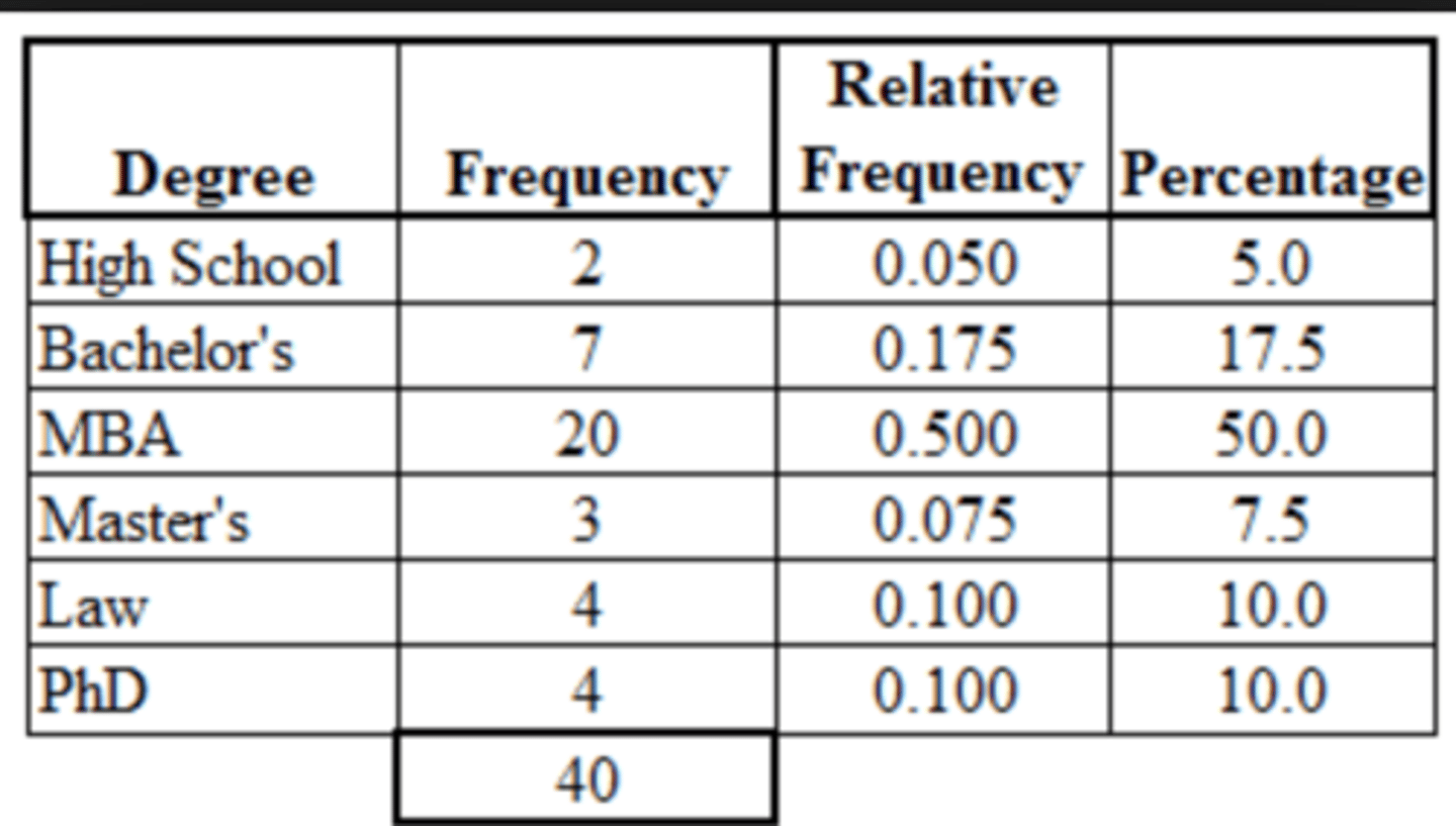
relative count/frequency

count/total = % or decimal

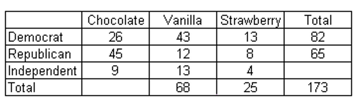
two way table

bar graphs

representing quantitative variables

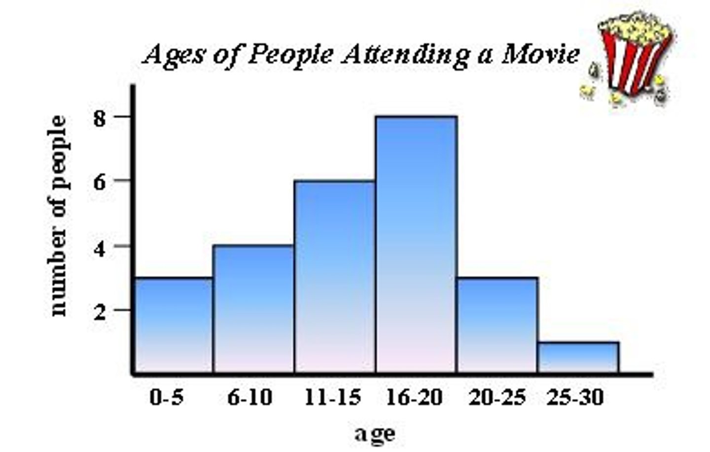
histograms

stem and leaf: stemplots, back-to-back stemplots

dotplots

cumulative relative frequency graphs (ogives)

histograms

(max - min)/number of bins

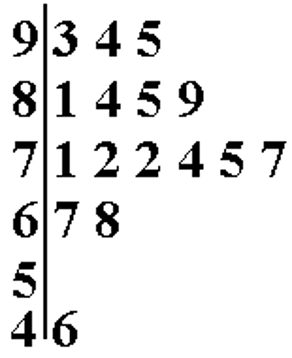
stemplots

DO NOT FORGET KEY

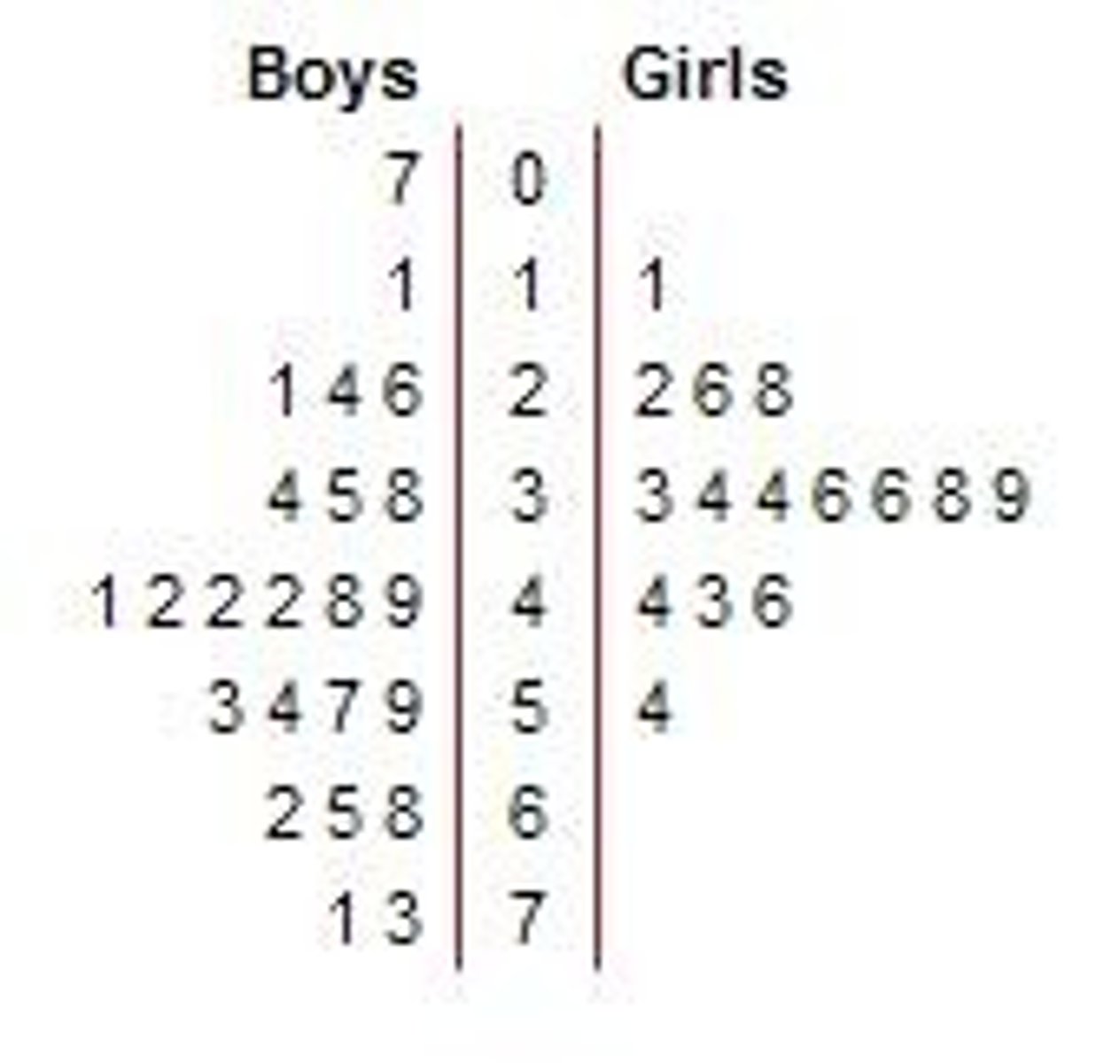
back-to-back stemplot

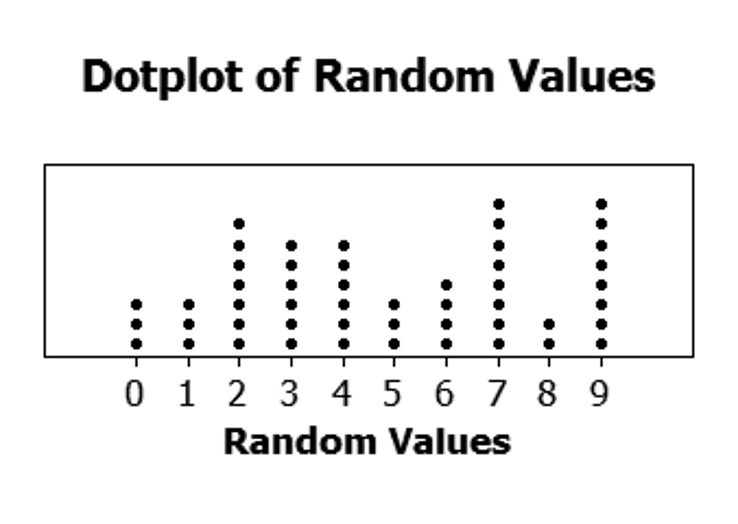
dotplots

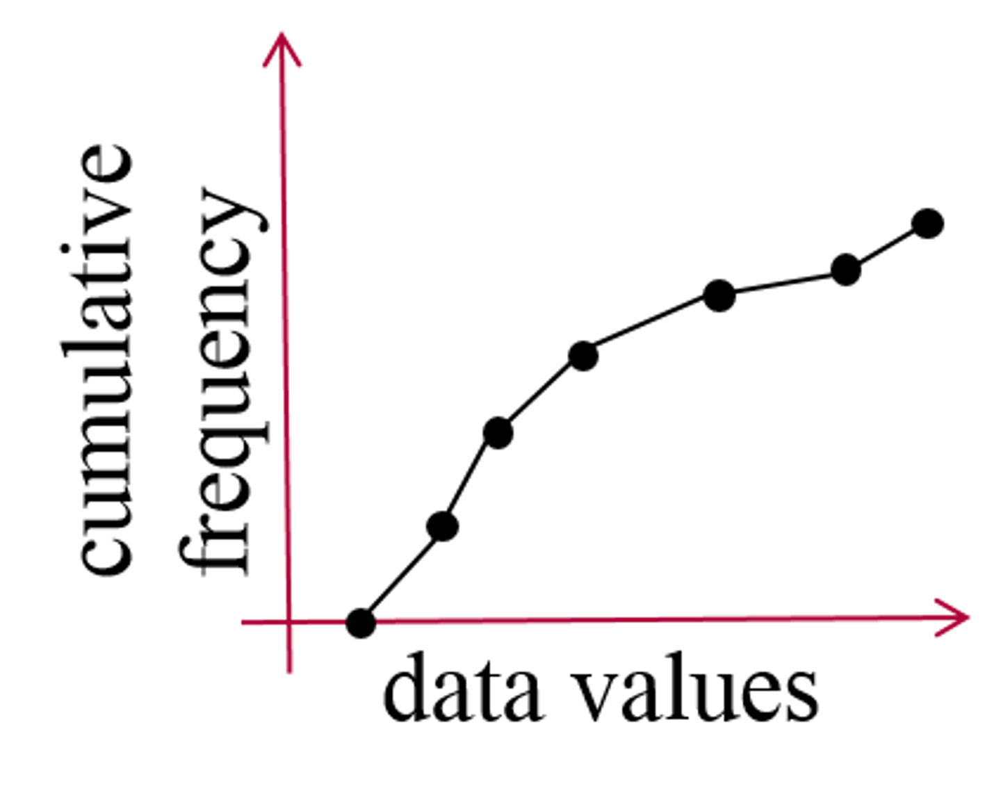
ogives

1. relative frequency

2. add percents together cumulatively

-> start at minimum x value not zero

percentiles

indicate the distance of a score from 0

ex) 99th percentile score = 99% people scored lower

describing distributions

SOCS (shape, outliers, center, spread)

-> quantitative values only

shape

unimodal, bimodal, uniform, symmetric, left skewed, right skewed

outliers

visual outliers, outlier tests, standard deviation rule

outlier test

Q1-1.5(IQR) lower

Q3+1.5(IQR) upper

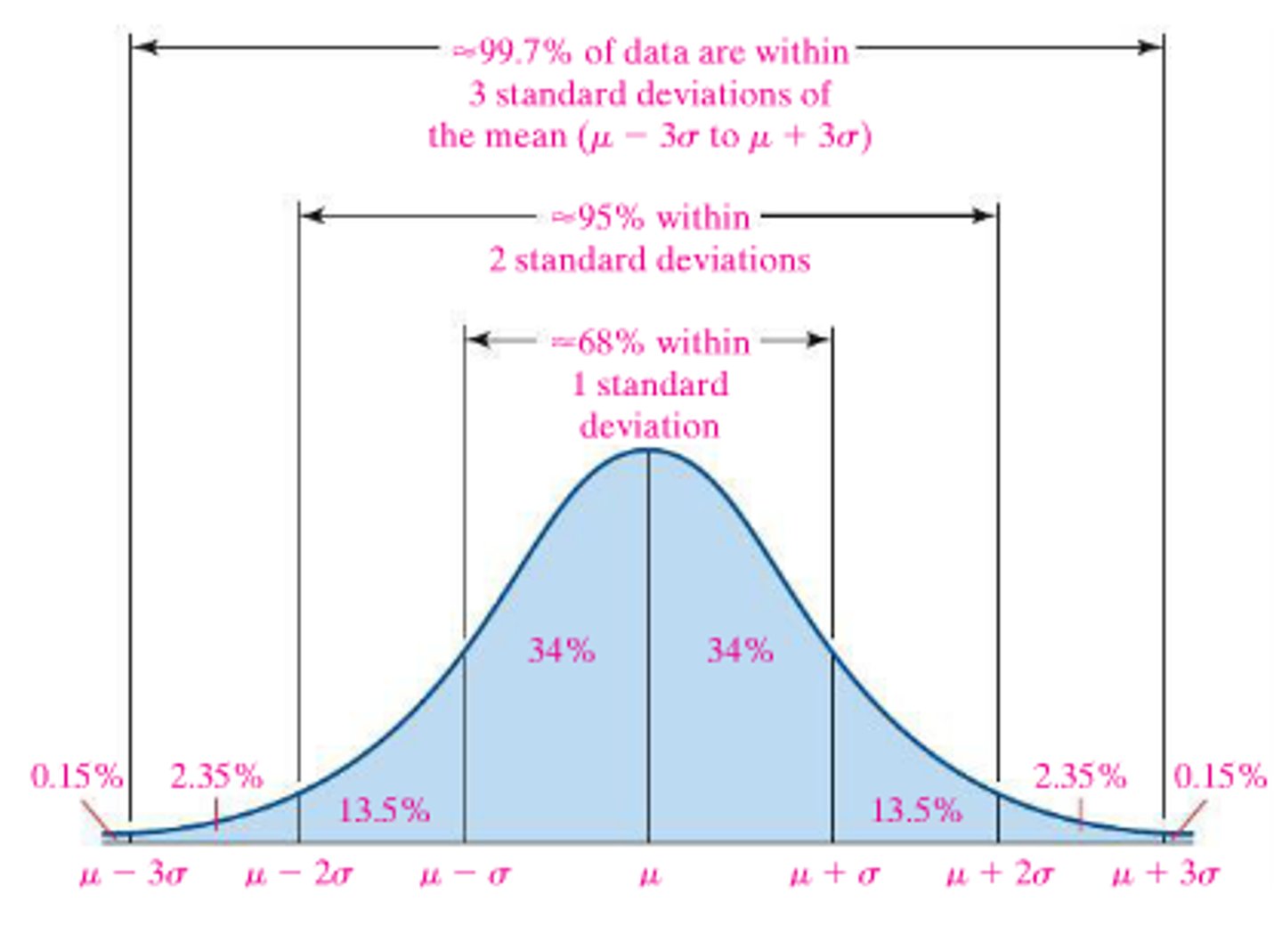
standard deviation rule

Mean +- 2*SD

center

mean, median, mode

non-resistant

mean

resistant

median, mode

center for left skewed

mean < median < mode

center for right skewed

mode < median < mean

spread

range, standard deviation, IQR

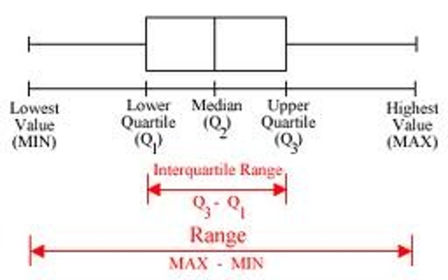
range

max - min = range

standrad deviation

average deviation of an observation from the mean

variance

(standard deviation)^2

greater standard deviation

greater variation

broader curve

center-spread pairs

standard deviation - mean

IQR - median

IQR

Q3-Q1

boxplots

"describe the distribution"

1. create your graph (categorical/quantitative)

2. summarize findings

"compare the distributions"

use comparison words (smaller, greater than, etc)

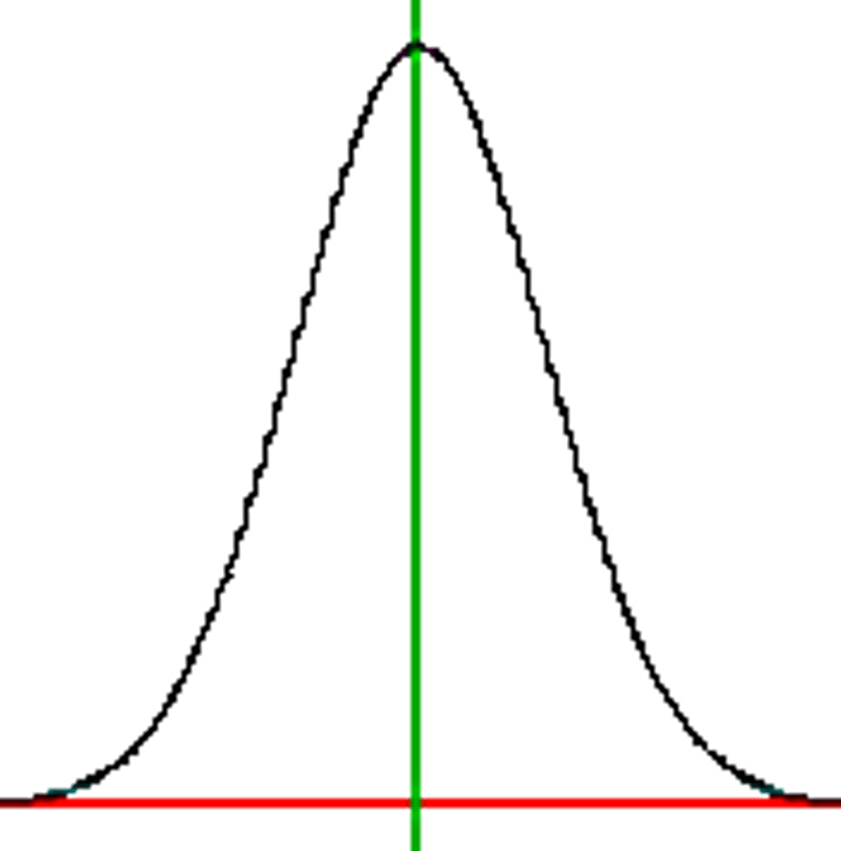
normal curve

A symmetrical, bell-shape that describes the distribution of many types of data

-> almost all data lie within 3 standard deviations

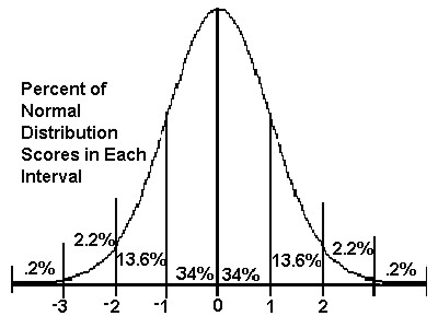
emperical rule

68-95-99.7

standardizing

making the mean 0 and standard deviation of 1 through z-scores, calculation of how far away an observation is from its mean

-> not just for normal distributions

z-score

(x-mean)/standard deviation

z-score interpertation

how many standard deviations you are away from the mean

ex) z-score of .67 means that score X is .67 SD away from the mean

standard normal curve

for any normally distributed curve

standard normal probability table

calculator-directions:

2nd -> vars

2: normalcdf(

percent of data below/between/above z-score of X

P(z < z score number)

calculator directions

SHOW probability, test name, numbers plugged into calculator

percent of subject below/between/above number X

P(x < number)

calculator directions

SHOW probability, test name, numbers plugged into calculator

comparison of below/between/above number X and z-score of X

give out same exact results

using z scores in word problems (for FRQs only)

P(x < number) = P (z < z score number)

percentages to z-score

(opposite of cards 46-49)

calculator directions:

2nd -> vars

3: invNorm(

percentages to raw data

1. percentile -> percentage below

2. calculator directions

3. plug in z score, mean, and standard deviation

4. solve for x

percentage lies BETWEEN distribution when

percentage to raw data

(1 - middle/symetrically orientated percentage)/2 = area