Biostats Unit 1

Inferential statistics

reach decisions about a large body of data if all we have is a small part

Data

raw material of statistics

Statistics

a field of study concerned with:

1) Collection, organization, summarization, & analysis of data

2) the drawing of inferences about a body of data when only a part of the data is observed

3) interpret & communicate results

• an estimated value calculated from a sample, varies from sample to sample

Where do we get data?

1) Routinely kept records

2) Surveys

3) Experiment

4) External sources

Variable

If a characteristic takes on different values in different persons, places, things

Quantitative variable

One that can be measured in the usual way & has units. Conveys info about an amount (does it make sense to find the avg?)

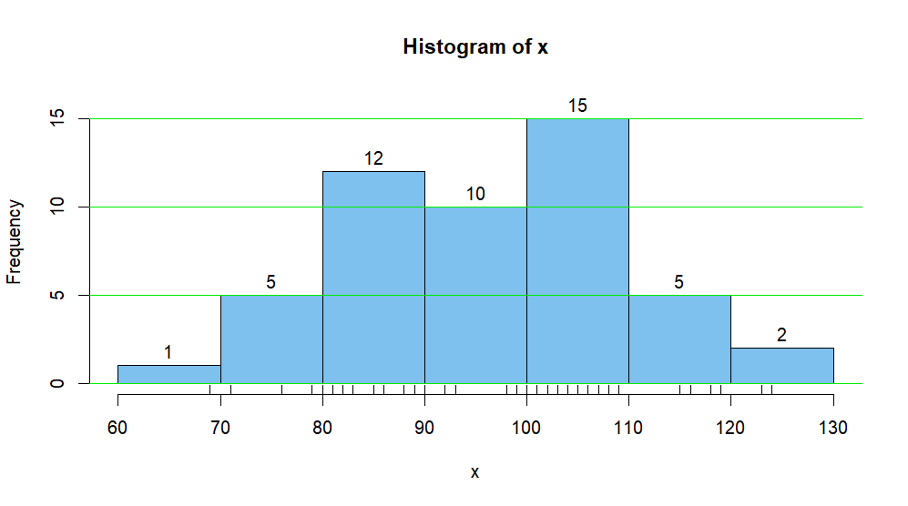
Best graphs:
✅ Histogram (especially for large data sets)
✅ Box-and-whisker (for comparing medians and outliers)
✅ Dotplot (good for small datasets)
✅ Stem-and-leaf (also good for small to medium datasets)

Qualitative variable

one that has categories

-we count the # in each category, called the frequency

exp: eye color, ethinic group, medical diagnoses

-Bar graph best for this type of data

Random variable

when the values arise as a result of chance factors & so can’t be predicted

Observations/measurements

Values from the measurement procedure

Discrete variable

characterized by gaps or interruptions in the values that it can assume

exp: coin flip (heads or tails)

-# of pts seen each day

Continuous random variable

-doesn’t posses any gaps or interruptions

-it can assume any value within a specified relevant interval of values

-e.g: weight, height, wrist circumference

Population

the collection of all entities for which we have an interest

-entities=cases=units

Population of values

-measurement of a variable on each of the entities we generate

N

size of the finite population (fixed # if values/entities)

Infinite population

if there are an endless # of values

Parameter (fixed #)

an exact value calculated from a pop

Sample

a part of the pop

-we use n=size of sample

Measurement

an assignment of #s to objects or events according to a set of rules

-various scales result from the different rules

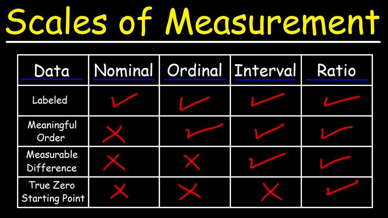
Nominal scale

• Definition: Categorizes data without any order or ranking.

• Examples: Gender, blood type, types of bacteria, colors.

• How to Identify: Look for data that are names, labels, or categories without a meaningful sequence.

Mutually exclusive

in 1 & only 1 category or group

Collectively exhaustive

all possible categories are listed

Ordinal scale

• Definition: Categorizes data with a meaningful order, but the intervals between categories are not equal.

• Examples: Pain severity (mild, moderate, severe), class rank, stages of cancer.

• How to Identify: Look for rankings or ordered categories where the difference between ranks isn’t uniform.

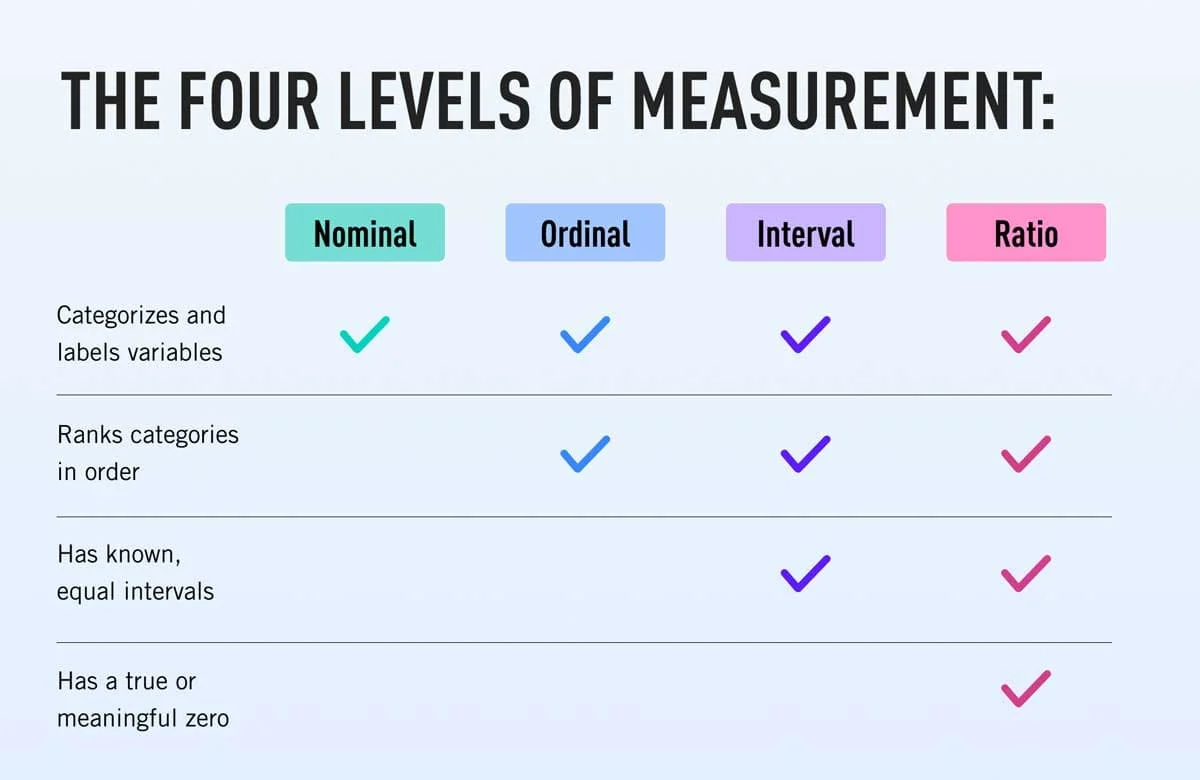
Interval scale

• Definition: Numerical data with equal intervals between values but no true zero point.

• Examples: Temperature in Celsius or Fahrenheit, dates on a calendar.

• How to Identify: Check for numeric data where subtraction makes sense, but there’s no absolute zero (e.g., 0°C doesn’t mean “no temperature”).

Ratio scale

• Definition: Numerical data with equal intervals and a true zero, allowing for meaningful ratios.

• Examples: Height, weight, age, enzyme activity, heart rate.

• How to Identify: Look for numeric data with a true zero (e.g., 0 means none of the quantity), and ratios make sense (e.g., 20 kg is twice as heavy as 10 kg).

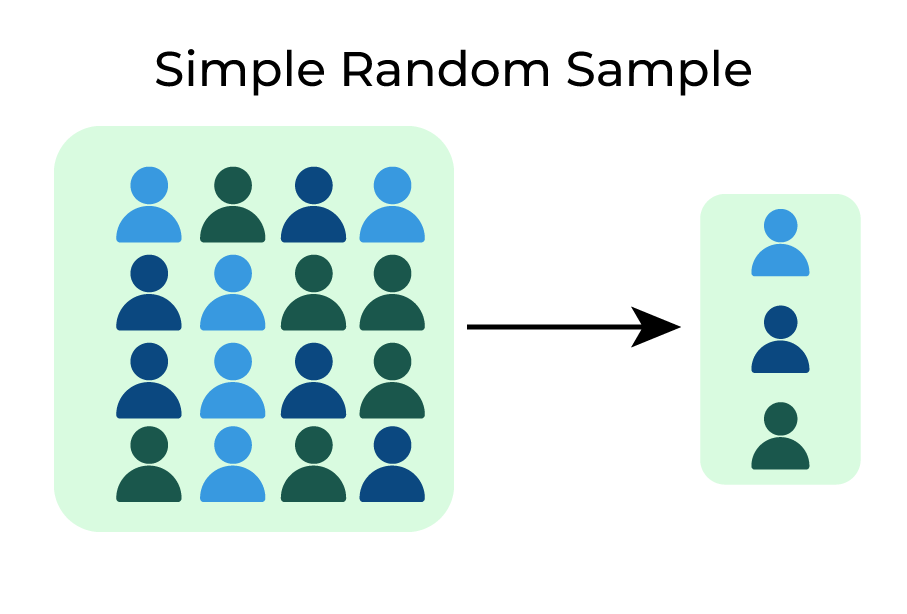
Simple random sample

If a sample of size n is drawn from a pop of size N in such a way that every possible sample of size n has the same chance of being selected

Sampling with replacement

every member of the pop is available at draw

-every member could be selected again (& again)

Sampling w/o replacement

we would not record the value of the variable for any member that has already been selected

-usually do this

Research study

a scientific study of a phenomenon of interest. Involves designing the sampling protocols, collecting & analyzing the data, & providing valid conclusions based on the analysis

Experiment

a special type of research study in which observations are made after specific manipulations of conditions have been done

Systematic sampling

used in health sciences calculate total number of records needed for study

-use a random # as starting point —> call it record x

-pick a second, calculated by # of records desired, to get the sampling interval, use K

-Data in sample: x, x + k, x +2k, etc.,

Scientific method

a process by which scientific info is collected, analyzed & reported in order to produce unbiased & replicable results in a effort to provide an accurate representation of the observable phenomena

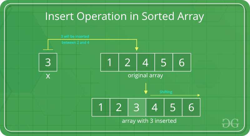
Ordered array

A listing of the values of a collection (set) in order of magnitude from smallest to largest (in population or sample)

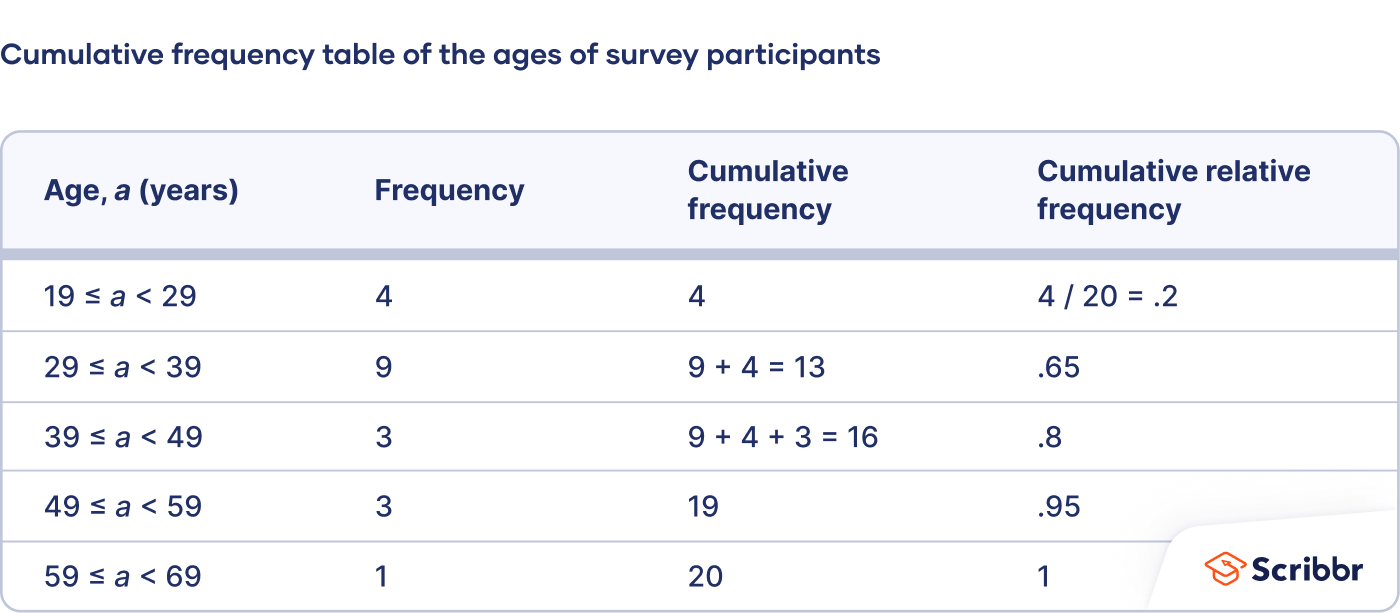
Relative frequency of occurrence

proportion of values falling in each class

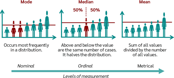
Measure of central tendency

a single value that is considered typical of the set of data, i.e, the “average” value

There are 3: mean (avg), median, mode

(Useful) properties of mean

1) Uniqueness: for a given set of data, there is 1 & only 1 mean

2) Simplicity: easy to calculate & understand

3) Since each & every data value is used (good), however extreme values can have an undue influence on the mean

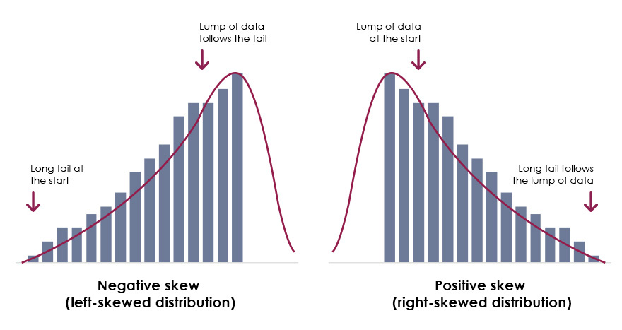
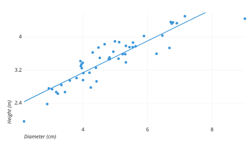
Skewed

If the graph (histogram or frequency polygon) of a distribution is asymmetric, the distribution is said to be

Positively skewed/skewed to the right

If a distribution is not symmetric because it has a long tail to the right, we say that the distribution is

-if the mean is greater than the mode

-the mean is larger than the median because the extreme high values pull the mean to the right, while the median remains near the center of the data.

Negatively skewed/skewed to the left

If a distribution is not symmetric because its graph extends further to the left than to the right, that is, if it has a long tail to the left, we say that the distribution is

-mean is less than mode

Dispersion

refers to the variety that they exhibit

-conveys information regarding the amount of variability present in a set of data. If all the values are the same, there is none; if they are not all the same, it is present in the data

-values are widely scattered—> it is greater

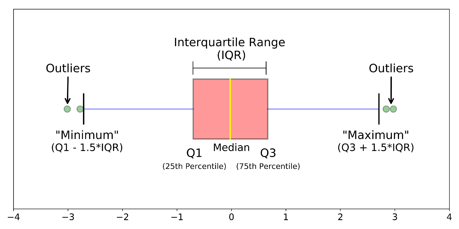
Interquartile range (IQR)

the difference between the third and first quartiles

-Q3-Q1

A large value indicates a large amount of variability among the middle 50% of the relevant observations, and a small value indicates a small amount of variability among the relevant observations

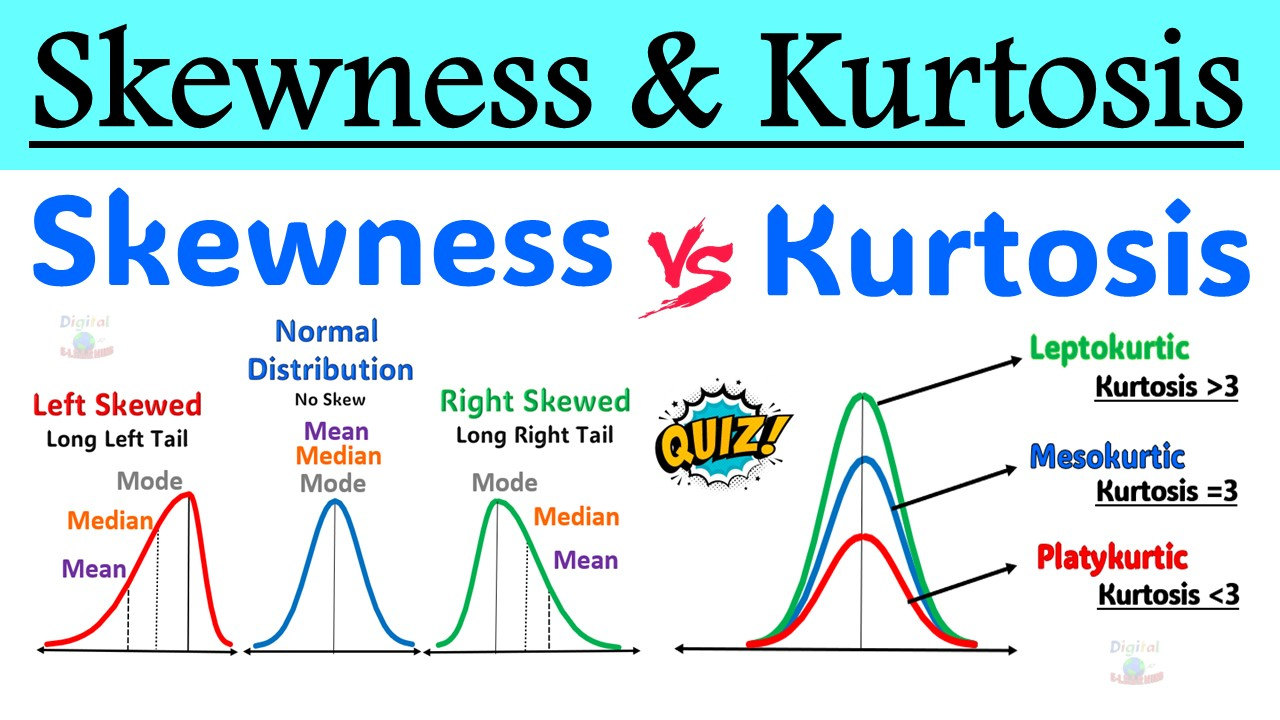
Kurtosis

a measure of the degree to which a distribution is “peaked” or flat in comparison to a normal distribution whose graph is characterized by a bell-shaped appearance.

Outlier

a data point that differs significantly from other observations

Objective probability

comes from objective processes

2 divisions: classical or relative frequency

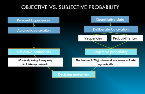
Classical probability

-(a priorirprobability) is based on counting theory & the idea that each event are equally likely to occur

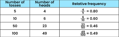
Relative frequency probability

( a posteriori or experimental)

is based on the repeatability of same process & the ability to count the # of repetitions & the # of times the event of interest occurs

Subjective probability

holds that probability measures the confidence that an individual has in the truth of a particular proposition. Does not need repeatability, can be used for an event that might only happen once

-We use Bayesian methods

Prior probability

of an event is probability based on prior knowledge, prior experience, or results from prior data collection

Posterior probability

of an event is probability obtained by using new information to update or revised prior probability

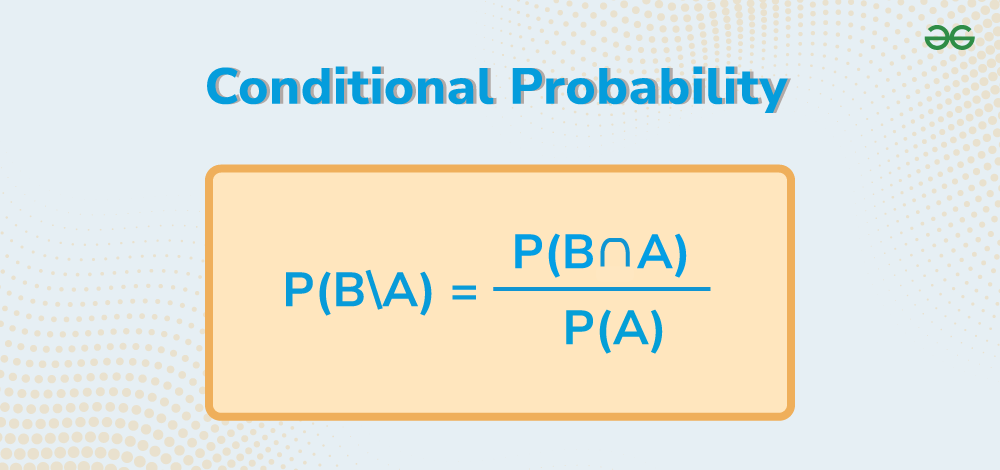
Conditional probability

When probabilities are calculated with a subset of the total group as the denominator

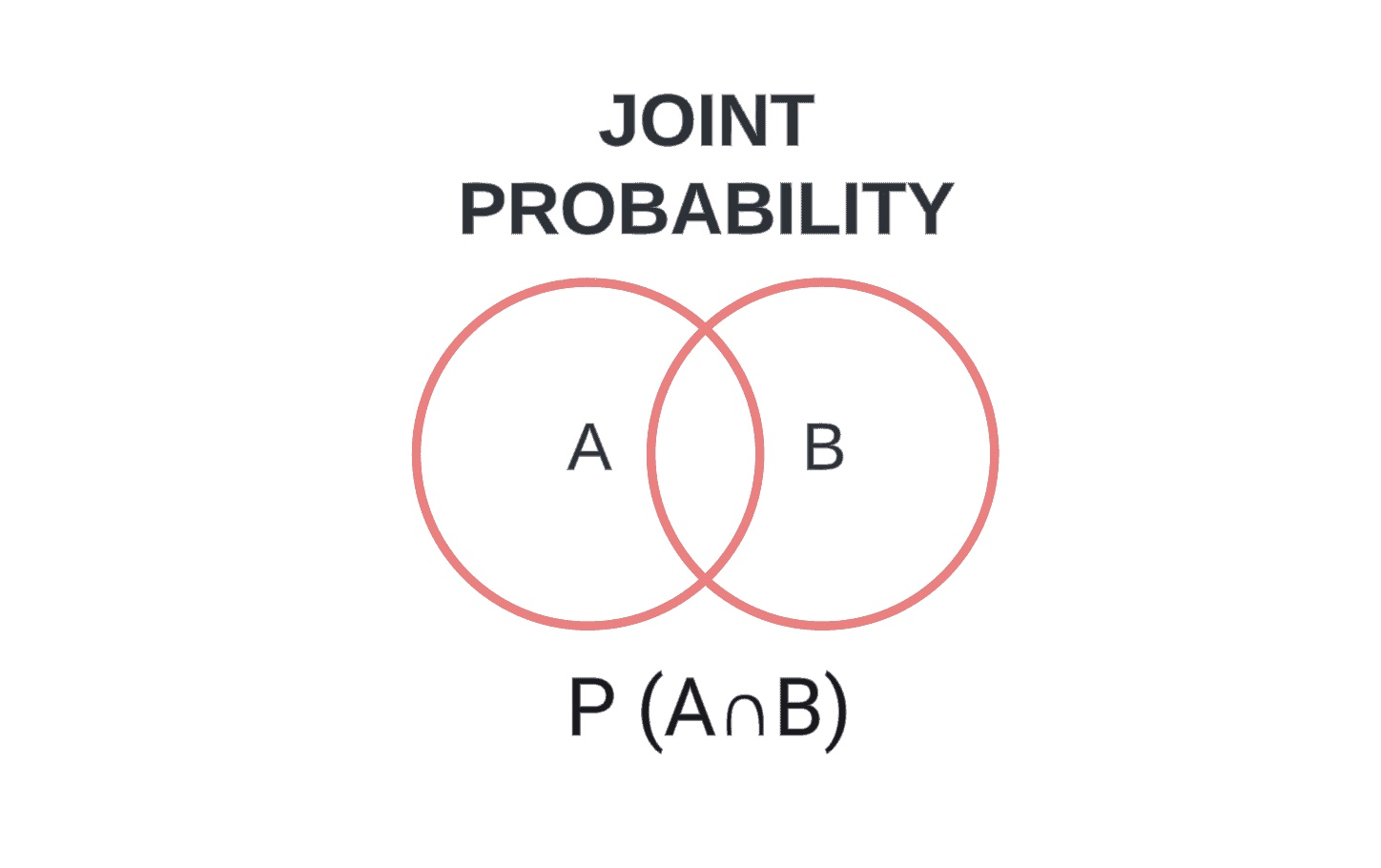
Joint probability

Sometimes we want to find the probability that a subject picked at random from a group of subjects possesses two characteristics at the same time.

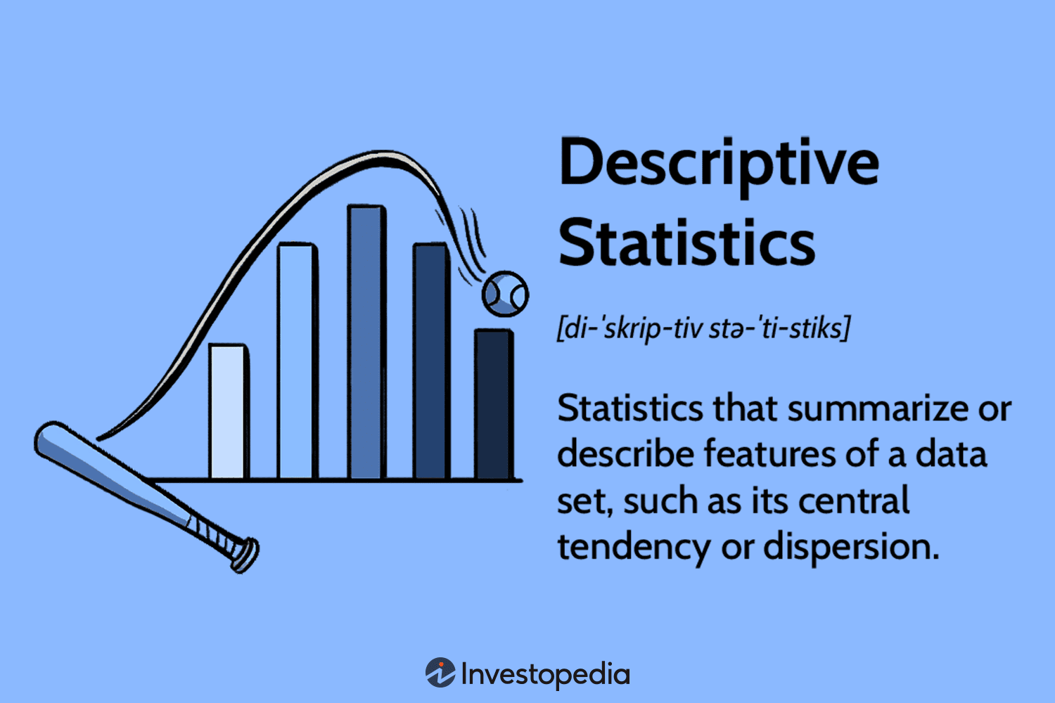
Descriptive statistics

provide simple summaries about the sample and about the observations that have been made. Such summaries may be either quantitative, i.e. summary statistics, or visual, i.e. simple-to-understand graphs.

Biostatistics

a field of study that uses statistical methods to analyze data related to living organisms.

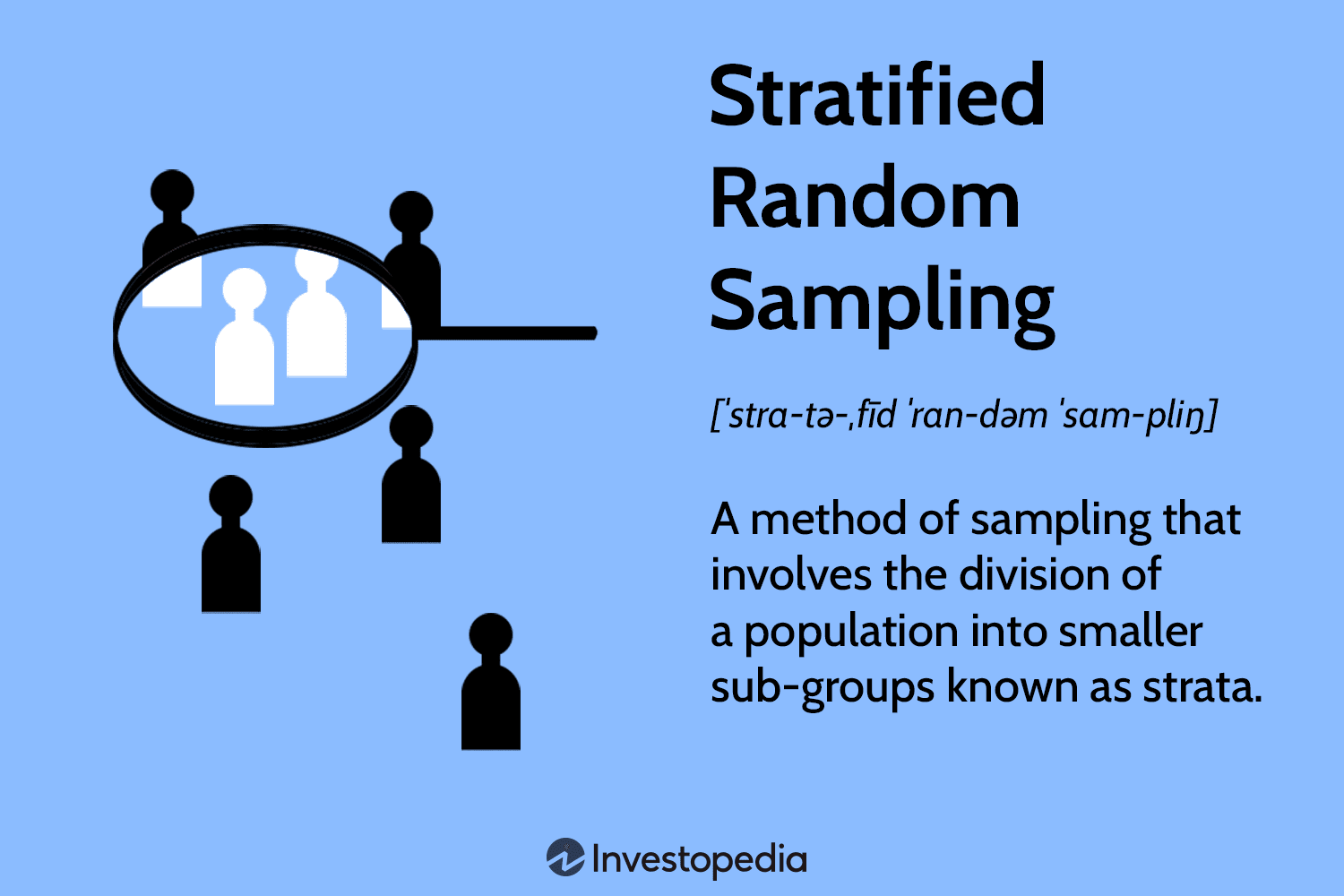
Stratified sampling

researchers divide subjects into subgroups called strata based on characteristics that they share (e.g., race, gender, educational attainment). Once divided, each subgroup is randomly sampled using another probability sampling method.

1. Identify Strata (Groups):

   • Group students by class standing: Freshmen, Sophomores, Juniors, Seniors.

2. Determine the Population Size (N):

   • N=100N = 100N=100 students.

3. Decide the Sample Size (n):

   • n=20n = 20n=20 students.

4. Determine the Proportion from Each Stratum:

   • Freshmen: 40/100×20=8 students.

   • Sophomores: 30/100×20=6 students.

   • Juniors: 20/100×20=4 students.

   • Seniors: 10/100×20=2 students.

5. Randomly Select Students from Each Stratum:

   • Randomly select 8 Freshmen.

   • Randomly select 6 Sophomores.

   • Randomly select 4 Juniors.

   • Randomly select 2 Seniors.

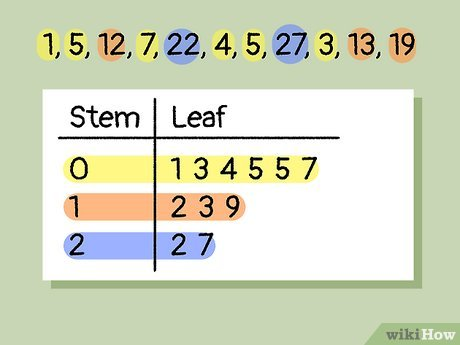
Stem-and-leaf display

a method of visualizing data by splitting each data point into two parts: a "stem" representing the leading digits and a "leaf" representing the last digit

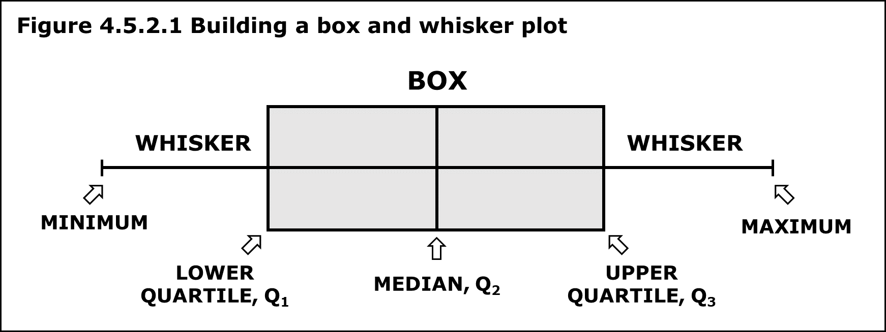
Box and whisker plot

a visual representation of data distribution that displays the minimum, first quartile, median, third quartile, and maximum values of a dataset using a box with lines extending outwards ("whiskers") to show the spread of the data, including potential outliers

Location parameter

a statistical measurement that indicates the center of a distribution

Common ones: 

• Mean: The most common location parameter, often represented by the symbol μ

• Median: The value in the middle of ordered values

• Mode: The most common value in a distribution

Frequency distribution

a graph or table that shows how often a value occurs in a data set.

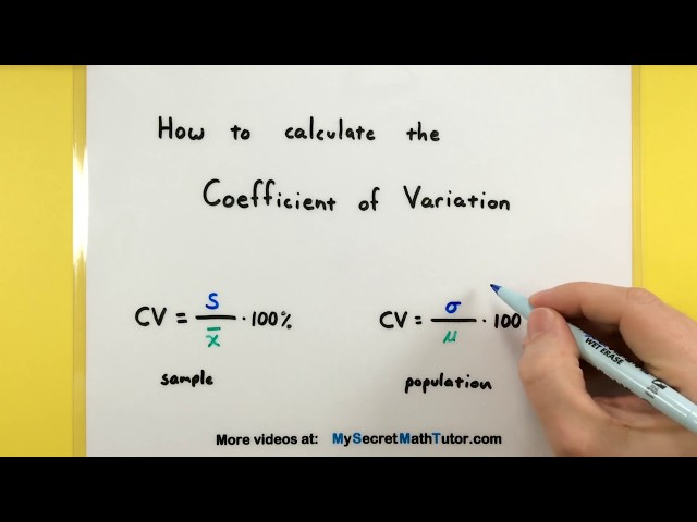
Coefficient of variation

the ratio of the standard deviation to the mean. The higher the value, the greater the level of dispersion around the mean. It is generally expressed as a percentage.

Box and Whisker outlier boundaries

• Lower Bound: Q1−1.5×IQR

  -anything below this number

• Upper Bound: Q3+1.5×IQR

  -anything above this number

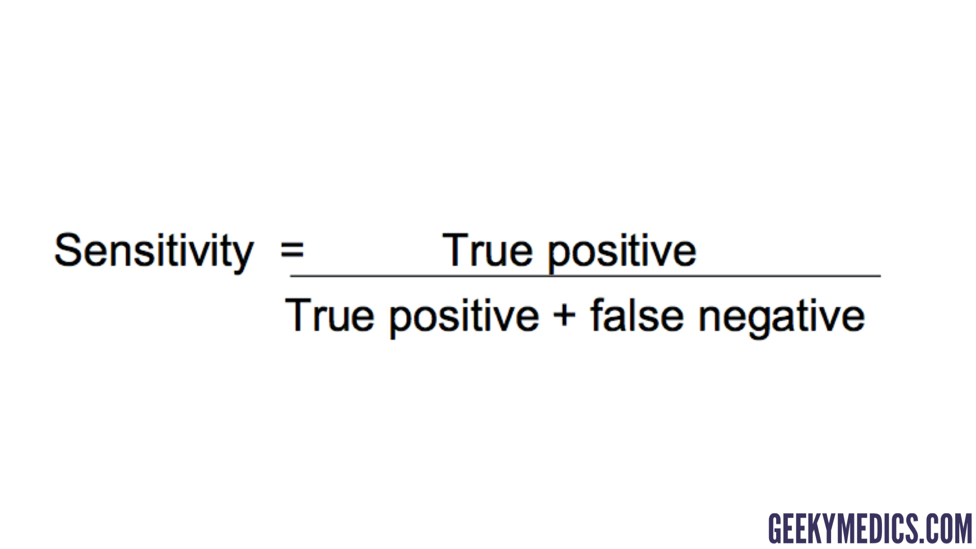
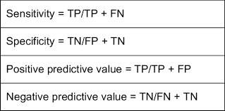
Sensitivity

a measure of how well a test can identify people who have a condition or outcome

=P(Test Positive | Has Disease)

= Number who tested positive and have disease / Total number who have disease

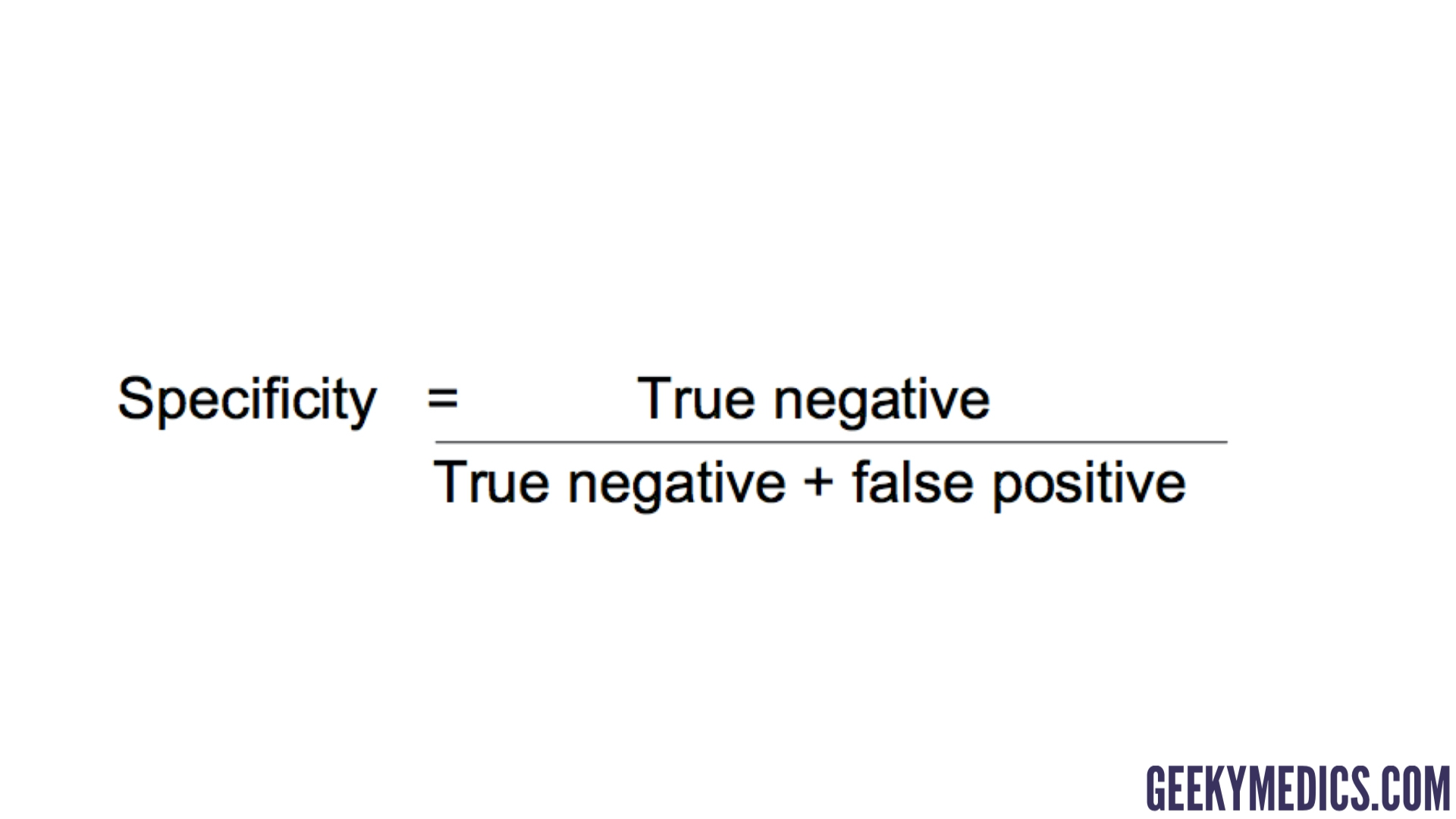
Specificity

a statistical measure of how well a test can identify people who do not have a condition

P(Test Negative | No Disease)
= Number who tested negative and don’t have disease / Total number who don’t have disease

Predictive value positive

a statistical measure that indicates the probability of a positive test result correctly identifying a disease or condition

Predictive value negative

the probability that someone with a negative test result is actually free of disease

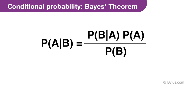
Bayes’ theorem

a mathematical formula that calculates the probability of an event based on prior knowledge

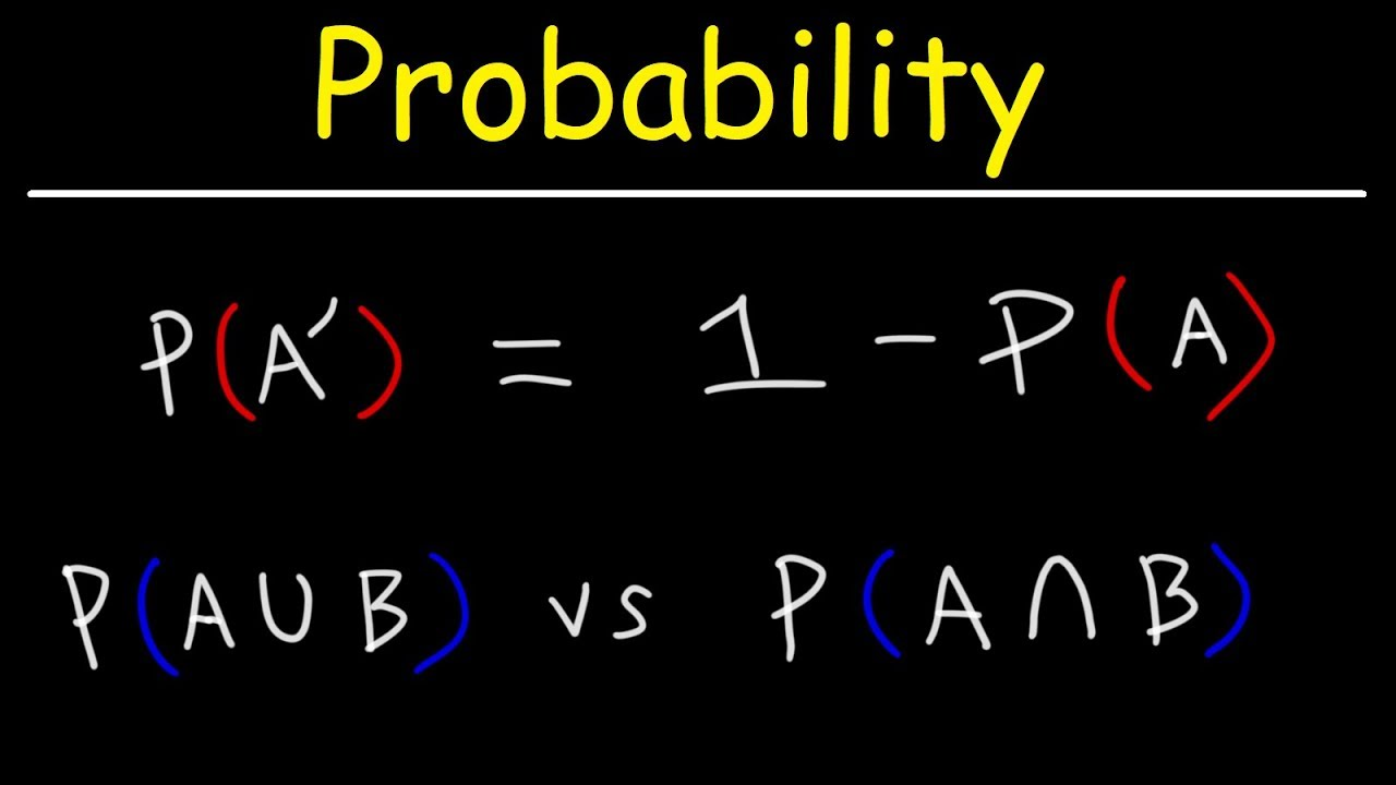
Complement probability

the probability that the event does not occur

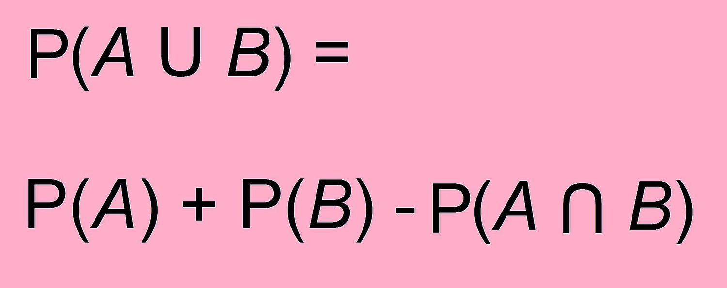
Addition rule

to find the probability of either event A or event B occurring, you add the individual probabilities of each event, then subtract the probability of both events occurring simultaneously

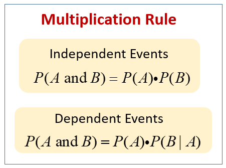
Multiplication rule

the probability of two (or more) independent or dependent events occurring together can be found by multiplying their individual probabilities.

Quick Test for Independence:

• Calculate P(A)×P(B).

• Compare it to P(A and B)

• If they are equal, the events are independent.

• If they are not equal, the events are dependent.

Class interval widths

1. Identify the Range of the Data

The range is the difference between the maximum and minimum values in your data set

2. Choose the Number of Classes

The number of classes (k) can be chosen based on guidelines such as Sturges' Rule:

k=1+3.322log⁡ n where n is the number of data points.

Alternatively, you can choose a reasonable number of classes (usually between 5 to 20, depending on the data size).

3. Calculate the Class Width

The class width (w) is calculated as:

w=Range/number of classes​

• Round up the class width to a convenient number for easy interpretation.

• If you get a decimal, round up to the next whole number to ensure full coverage.

Measurement scales

1. Nominal Scale

• Definition: Categorizes data without any order.

• Characteristics:

  • Names, labels, or categories only

  • No ranking or meaningful order

  • Can't do arithmetic on them

• Examples:

  • Gender (male, female, other)

  • Blood type (A, B, AB, O)

  • Eye color (blue, brown, green)

🔸 2. Ordinal Scale

• Definition: Categorizes data with a meaningful order, but the differences between categories are not measurable or consistent.

• Characteristics:

  • Ranked or ordered

  • Intervals are not equal or meaningful

  • Arithmetic is not valid

• Examples:

  • Survey ratings (satisfied, neutral, dissatisfied)

  • Education level (high school, bachelor's, master's)

  • Class rankings (1st, 2nd, 3rd)

🔹 3. Interval Scale

• Definition: Numerical data with meaningful differences between values, but no true zero point.

• Characteristics:

  • Ordered and equally spaced

  • No absolute zero (zero does not mean "none")

  • Ratios don’t make sense

• Examples:

  • Temperature in °C or °F (0° ≠ "no temperature")

  • IQ scores

  • Dates on a calendar

🔸 4. Ratio Scale

• Definition: Like the interval scale, but has a true zero, so ratios are meaningful.

• Characteristics:

  • Ordered, equal intervals, and a true zero point

  • All arithmetic operations are valid

• Examples:

  • Age

  • Height

  • Weight

  • Distance

  • Time duration

  • Money

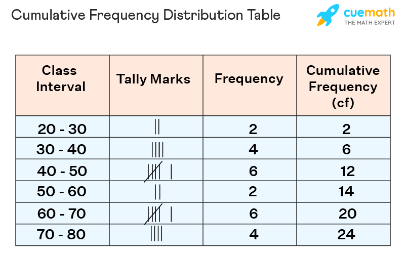
Cumulative frequency

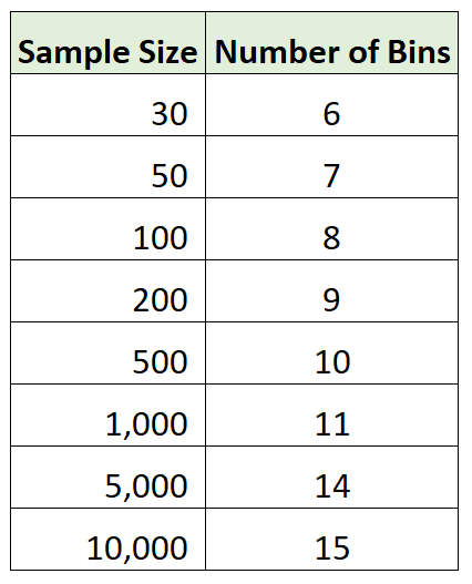
Sturges rule

-an equation to help one choose the number of bins in a histogram or frequency distribution which helps organize the data into a clear representation without it being too broad or too restricted

Which graphs provide a smooth vision of the data?

Histogram & Box and whisker

Which graph best shows interval spacings between data points?

dot plots

Which graph(s) can handle a large amount of data over a large range of values?

-Stem & Leaf

-Histogram

-Box & whisker

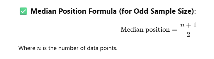
Median position for odd sample sizes

P(AUB) (“or” probability)

= P(A) + P(B)- P(ANB)

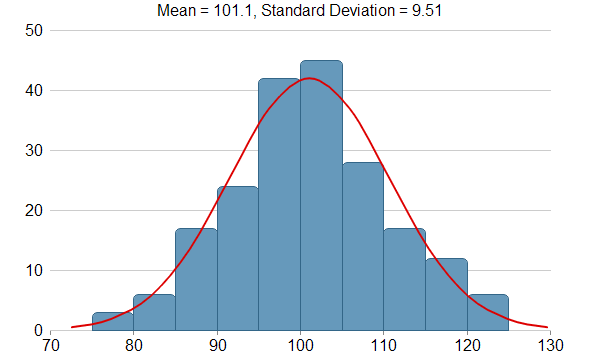
Bell shaped graph

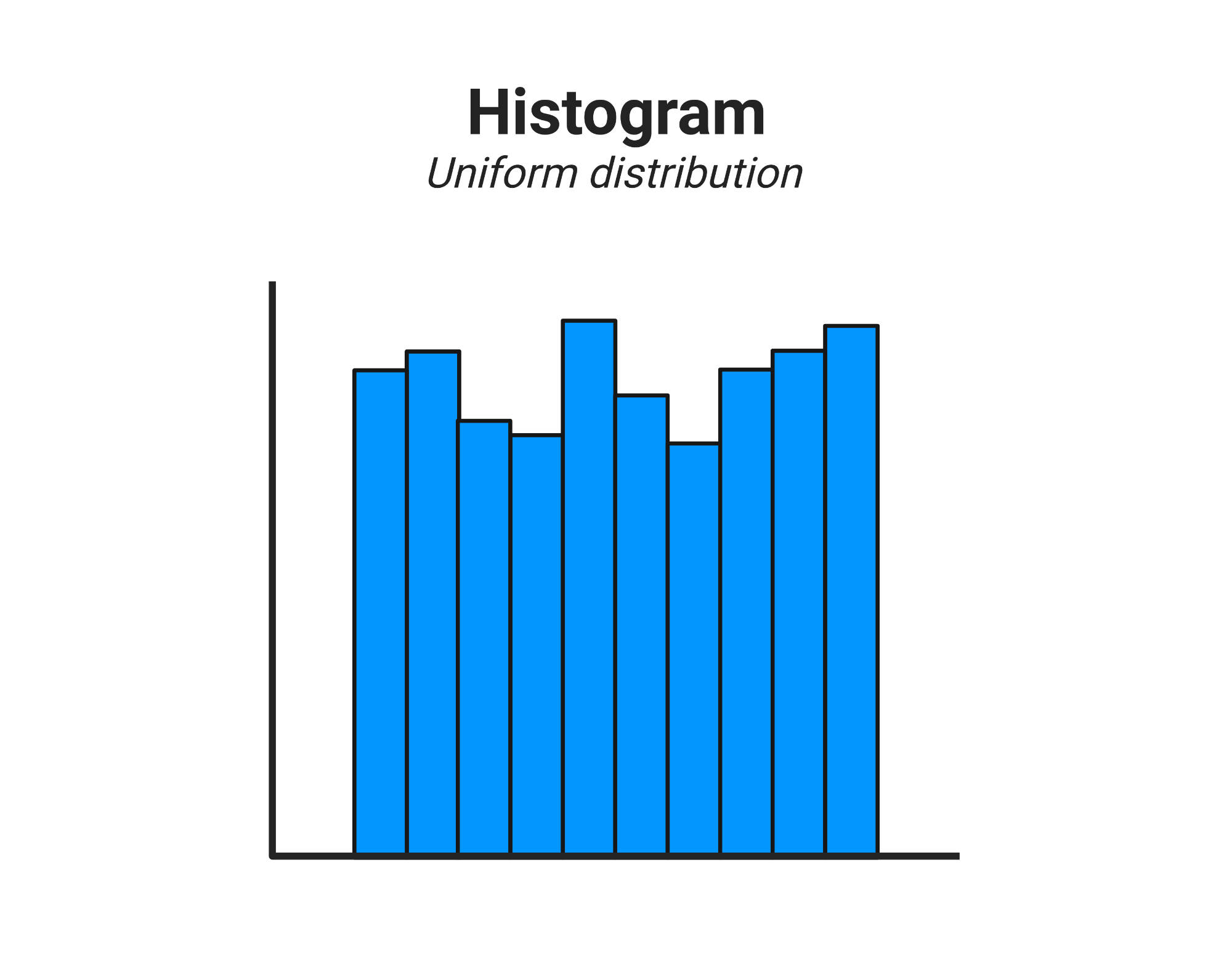
Uniform histogram

False positive

= P(Test Positive | No Disease)
= Number who tested positive but don’t have disease / Total number who don’t have disease