microeconomics graphs

all the graphs i need to know

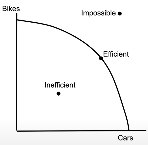
production possibilities curve

• shows you can produce two different goods

• any point outside the curve is impossible

• any point inside the curve is inefficient

• any point on the curve is efficient, as you are using all resources to the fullest

  • find the point on the curve that is most efficient for the socially optimal quantity (the quantity that society actually wants)

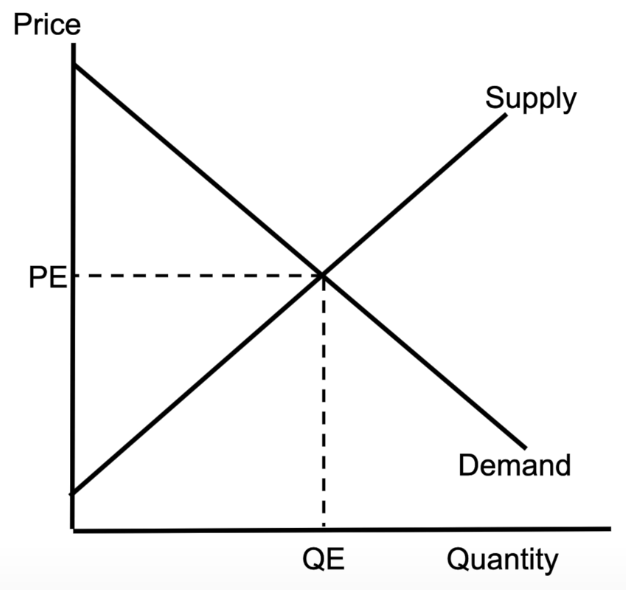
supply and demand

• supply and demand showing a competitive market

• shows equilibrium

• curve shifting

consumer vs producer surplus

• consumer surplus: what people are willing to pay for a good - what they actually pay

• producer surplus: what people actually pay vs what suppliers wanted to sell it for

• total surplus = sum of both

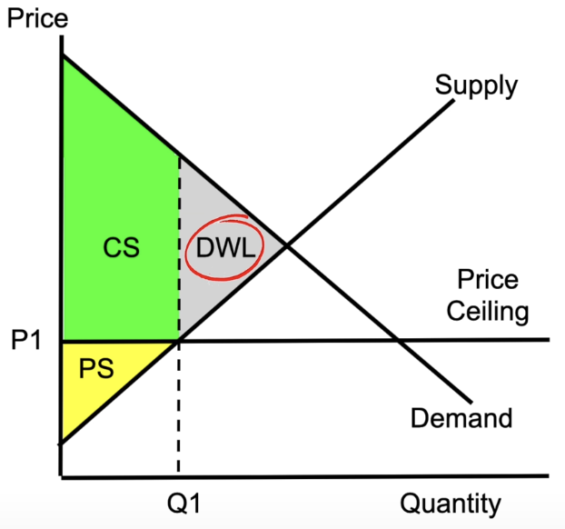
supply and demand with a price ceiling

• eg. government limits the maximum price

• causes a smaller producer surplus and larger consumer surplus

• creates dead weightloss: the idea that we aren’t producing the socially optimal quantity (producing less than they want)

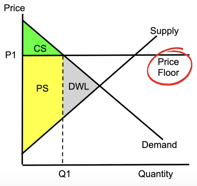
supply and demand with a price floor

• eg. the price can’t fall below a certain point

• causes smaller consumer surplus and larger producer surplus

• creates dead weight loss: producing more than they want

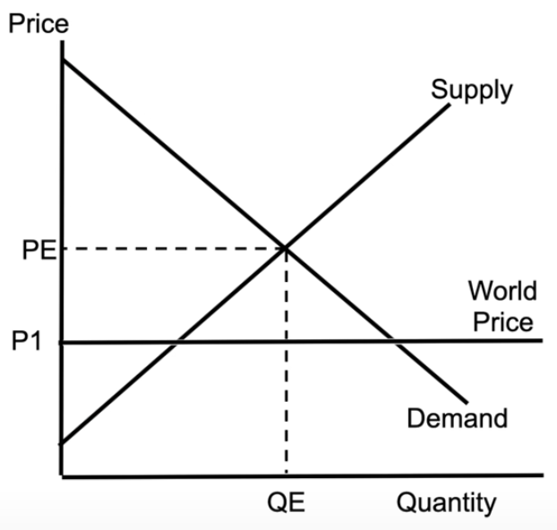
supply and demand showing result of trade

• shows result of international trade

• PE = domestic price of the product

• P1 = the price we can get it for, if we buy it from other countries

• no dead weight loss, which explains why economists like international trade

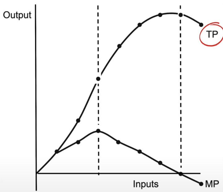
short-run production function

• TP = total product = total amount produced

• as you hire more workers TP increases at an increasing rate, then increases at a decreasing rate, then eventually starts decreasing

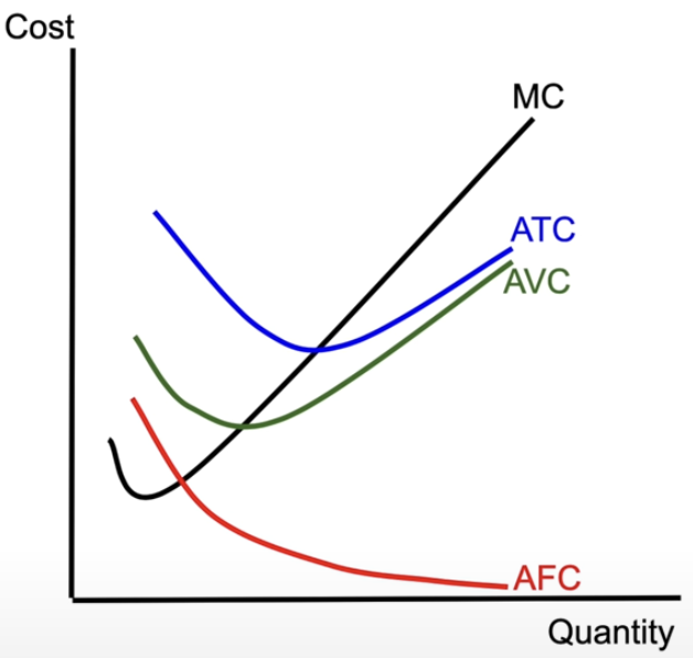
short-run per unit cost curves

• MC = marginal cost → decreases then increases

  • tells you how much to produce

• ATC = average total cost - decreases, hits a minimum, then increases

  • tells you how much profit or loss you’re making per unit

• AVC = average variable cost → nears ATC

• AFC = average fixed cost → asymptote heading toward y = 0

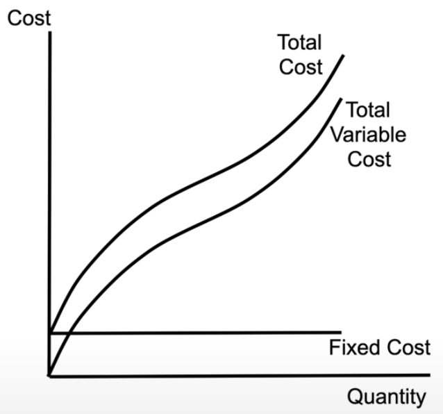
short-run total cost curves

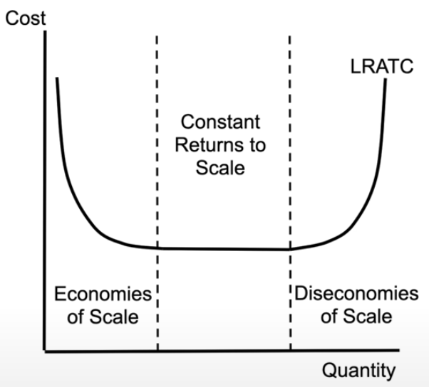
long-run average total cost curves

• in the long run, if all of our resources are variable, we end up with this

• shows all the sum of all short run curves

• economies of scale = as a company produces more goods or services, the average cost per unit decreases

• constant returns to scale: when you increase inputs to a production process by a certain proportion, the output will increase by the same proportion

• diseconomies of scale = average cost per unit of production increases as its output increases

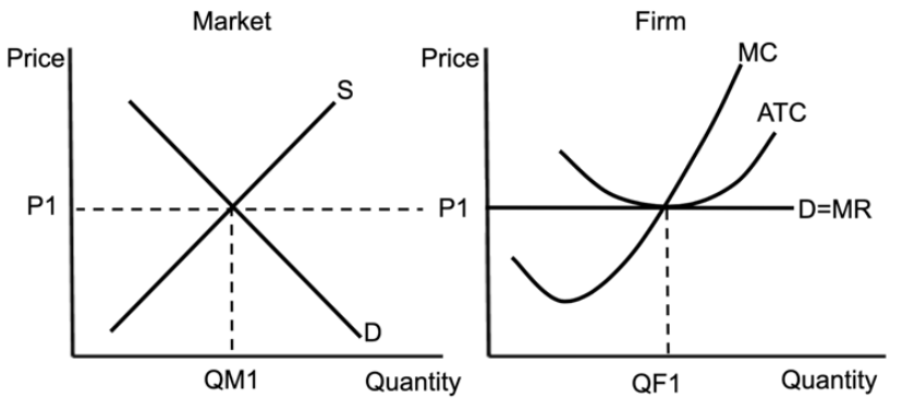
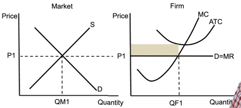
perfect competition (long run)

• P1: the price is set by the market (price takers) → horizontal demand = marginal revenue curve

• add in MC and ATC from short-run per unit cost curves

• shows perfectly competitive firm in long-run equilibrium

• you always produce where MR = MC → represents the profit maximising quantity

  1. producing where price = marginal cost → producing amount society wants

  2. producing at the lowest possible cost → producing productively efficient quantity

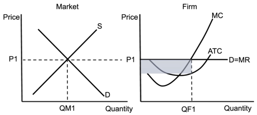
perfect competition short-run profit

• the blue part

perfect competition short-run loss

• the yellow part

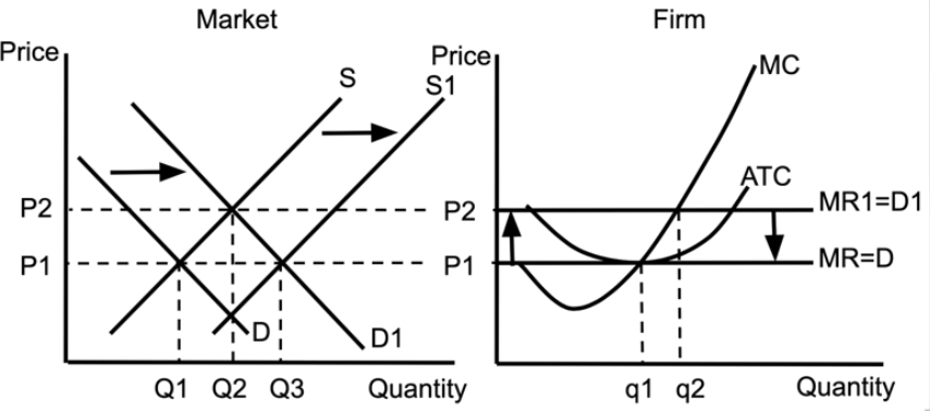
perfect competition from long run to short run back to long run

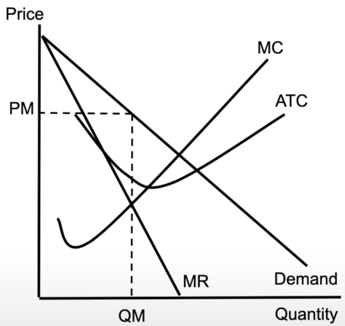
non-price discriminating monopoly

• downward sloping demand curve

• downward sloping marginal revenue curve

• MC and ATC stay the same shape

• still produce where MR = MC

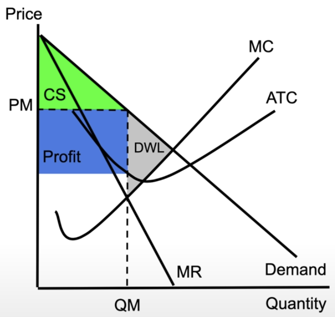
monopoly making profit

• a monopoly is not allocatively efficient

• not producing what society wants

• it holds back production to maximise profits

monopoly making loss

monopolistic competition in the long run

• ATC is tangent to the demand curve, showing no economic profit in the long run

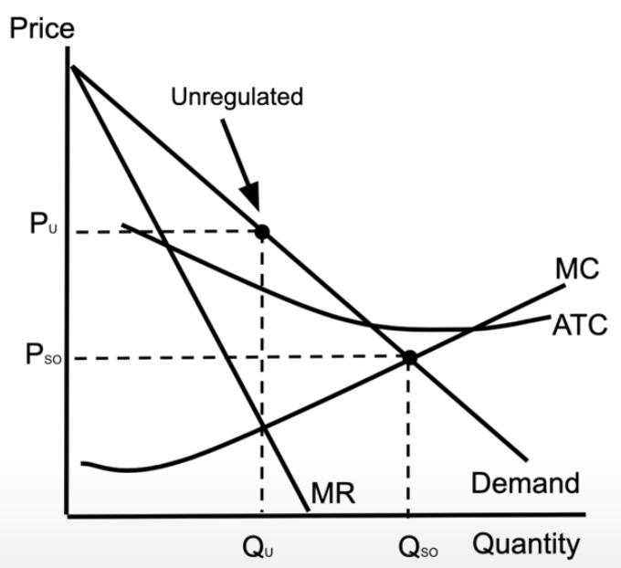
natural monopoly

• where the MC hits the demand curve (= the socially optimal quantity), the ATC is still falling

• this means that the firm can produce the product at the lowest possible cost

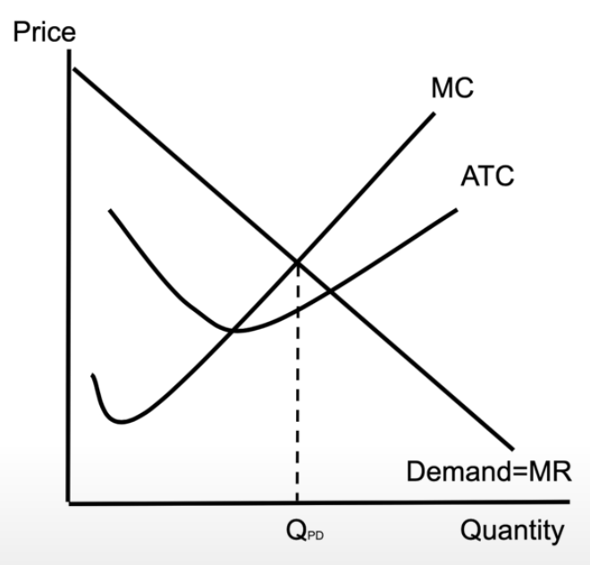
price discriminating monopoly

• the monopoly is charging each consumer exactly how much they are willing to pay

• demand curve = marginal revenue curve, and there is no consumer surplus → all of it becomes profit

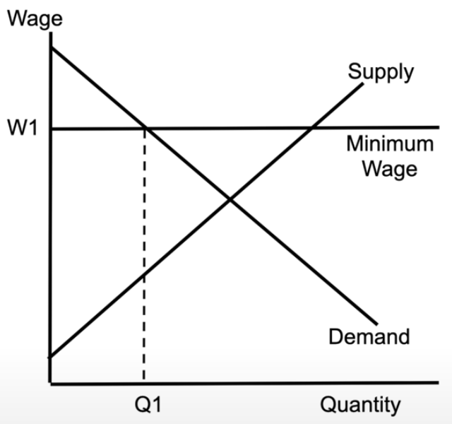
labour market (minimum wage)

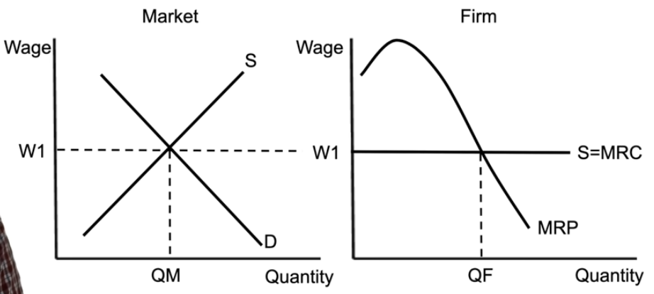
perfectly competitive resource market and firm

• perfectly competitive firm in the resource market = a firm hiring workers

• the wage for the firm is set by the market, gives you a horizontal supply curve, which = marginal resource cost

• marginal revenue product = how much each worker generates → downward sloping, tells you exactly how many workers to hire (where MRP = MRC)

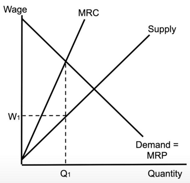
monopsony

• there is only 1 firm hiring, so the supply of labour is upward sloping

• there is an upward sloping marginal resource cost

• you hire where MRC = MRP

• the wage is below the equilibrium wage that would exist at perfect competition

• firms that hire workers at a lower wage, because they are the only firm hiring

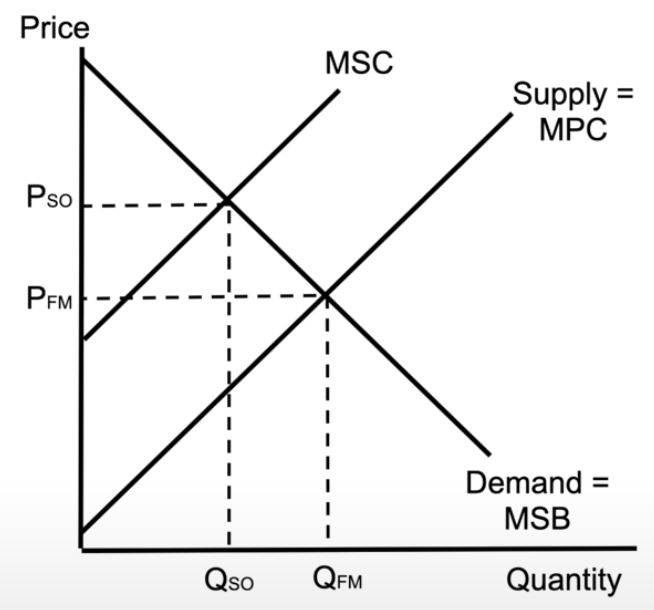
negative externality

• supply and demand show you the quantity produced in the free market → the free market quantity is wrong

• if this product creates a negative externality and there is additional costs on society, we end up with a marginal social cost (MSC)

  • MSC hits marginal social benefit, which shows the socially optimal quantity, which is less than the free market is making

  • result: dead weight loss (overproducing, because we didn’t take into account the additional costs on society)

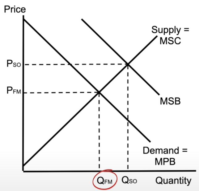
positive externality

• quantity of the free market is less than the socially optimal quantity

• not factoring in all the additional benefits that society gets from the product

• dead weight loss → the free market is underproducing something that society wants more of

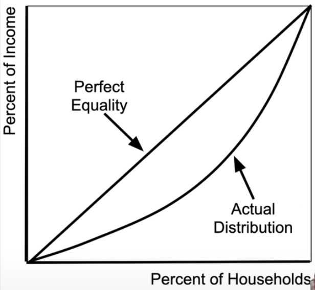
lorenz curve