Stats 1

categorical data

factor, nominal

no particular relationship between the different possibilities

can’t average them/do maths

eg. job, eye colour, drink preference

continuous data

interval

can do maths

eg. weight, height, reaction time, test score

ordinal data

ordered categorical, factor, likert scale

an order to the sequence

can’t do maths

can talk about frequencies but not averages

eg. grades, how religious someone is

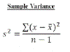
descriptive statistics

central tendency: mean, mode, median

variability: range, variance, standard deviation, interquartile range

they describe what’s going on in the data/sample (not the larger population)

mean

average

for continuous data

sum of all values divided by number of values

outliers are a weakness (anomalies)

can be influenced by very high/low scores

mode

value that happens most often

for continuous/categorical data

one = unimodal

two = bimodal

median

the middle number

for continuous data

sort data in ascending order and find number

can only have one

variability

how spread out the data are

how far away from the mean/median the data points are

only suitable for ordinal/continuous data

range

highest value - lowest value

know the boundaries of our data

useful to detect outliers/data input errors

doesn’t tell how common really high'/low numbers are

variance

how far numbers are spread out from the mean

feeds into other statistics that makes it more useful

= (distance of scores from the mean) / (number of scores - 1)

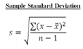
standard deviation

square root of the variance

describes variability within a single sample - descriptive

measure of average distance of each point from the mean, in the original units

small = data points close to mean

large = data points far away from mean

used to understand the variability in continuous/ordinal data

interquartile range

split our data into quarters (each contains 25% of the data points)

• put data into ascending order

• find the median (Q2)

• find the median of the first half (Q1)

• find the median of the last half (Q3)

• Q3 - Q1

the range (max-min) is the middle 50% of data

useful as it isn’t affected by outliers

when an odd number of data, find median, then in first half find the median while ignoring the Q2

histograms

use these to graphically visualise the frequency distribution of continuous data (eg. heights, weights, depression, reaction time)

make bin categories and then a frequency table, with frequencies of values in each bin

frequency on Y axis

the mode is the bin with the tallest bar

useful to see the shape/distribution of the data

tukey boxplot/box and whiskers

used to visualise continuous data and provide statistical summaries of data

shows 5 descriptive statistics in one plot

• minimum bound

• quartile 1

• median (Q2)

• quartile 3

• maximum bound

• plus outliers (statistically different to rest of data)

elements:

• interquartile range = Q3-Q1

• min and max bounds (not the true minimum and maximum, but the largest data points above and below the thresholds

thresholds in a boxplot

Q1 – (1.5xIQR)

Q3 + (1.5xIQR)

interpreting a boxplot

each section contains 25% of the data

shorter whisker = data will be quite similar (less variability)

longer whisker = data will have more variability

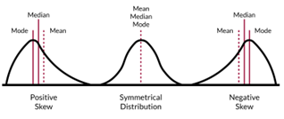
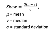
skewness

asymmetry is caused by the presence of extreme values that distort the shape of the data, which is why symmetrical distributions are quite rare

characterised by a long gentle tail on one side of the distribution and a shorter steeper tail on the other

about horizontal shape of distribution

negative skew - less than -2

normal skew - 0 (between -2 and +2)

positive skew - more than 2

symmetrical distribution

same shape on both sides (bell curve)

mean, mode and median very similar

in a box plot, the median line is central with equal proportions throughout

negative skew

longer tail slopes to the left

mean is lower than the median, which is lower than the mode

in a box plot, median and upper whisker are closer to the right/top

less than -2

positive skew

longer tail slopes to the right

mode is lower than the median, which is lower than the mean

in a box plot, median and lower whisker are closer to the left/bottom

more than 2

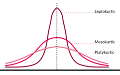
kurtosis

used to describe the shape of a distribution

an indicator of the number of extreme values in data

3 categories:

• mesokurtic - 3, conforms to classic bell curve shape

• platykurtic - less than 3, flatter profile with shorter tails indicating fewer outliers

• leptokurtic - more than 3, narrower center and longer tails indicating more outliers

kurtosis between 1 and 5 is within acceptable limits of normality for a given distribution (-2 and +2)

calculating skew by hand

Pearson’s coefficient of skewness

negative number = negatively skewed

positive number = positively skewed

skew of 0 = symmetrical data

bimodality

2 modes

not shown well in a box plot, so making a histogram is useful to show the distribution of the data properly

plotting extreme values

general weirdness

need to consider context of extreme values

robust statistics

the median

less vulnerable to distortion by extreme values

for some data, the median will provide a better estimate of central tendency than the mean

interquartile range less vulnerable too

non-robust statistics

the mean

extreme values can have a noticeable effect on it

SD also vulnerable to distortion by outliers, as it’s calculated using the mean

population

the entire group of individuals or items that a statistical analysis aims to describe or draw conclusions about

all the hypothetical individuals we want to understand something about

isn’t just all physical people currently existing, but a more abstract concept of all infinite individual that have/could exist

sample

randomly chosen individuals from the population who we test/study, which we assume represent the whole population

in reality, many samples are not random when studies are volunteer = bias (random is ideal though)

can calculate descriptive statistics to understand the sample, but these only describe the sample not the wider population

larger the sample size, the more precise the estimates about the population will be

statistical model

a mathematical and simplified representation of observed data/behaviour/reality, used to make predictions or draw inferences about the sample and generalise to the whole population

simplifies reality/complex matters to understand relationships between variables

all models are wrong - they are representations of a thing that doesn’t necessarily capture all the complexity of reality but are still useful to use eg. London underground map

perfect correlation model:

• data perfectly linear

• data would all lie on line of best fit

• can work out one variable if we know the other

can be relatively confident our model is reliable and appropriate for our data by understanding the assumptions it makes

if we reduce the discrepancy between the assumptions and our data, our model allows us to draw useful conclusions about the process that generates our data

they are also machines eg. the Rube-Goldberg machine (intentionally designed to perform a simple task in an overly complicated way

simple model

describing central tendency and variability in a measure

complex model

big network of how different variables connect to each other

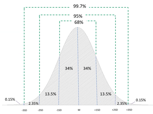
normal distribution

a probability distribution as a bell shaped curve

1 peak (mean, median, mode are equal)

can use SD as a unit of measurement (a data points distance from the mean can be measured using a number of SDs)

eg. histograms

defined by its density function (density plots)

follows the 68-95-99.7 rule

properties:

• symmetric about the mean/centre

• tail never hits 0

• characterised by mean and SD

• X in continuous

  • Y is defined for every value of X

  • what gives the curve its’ smoothness

  • ranges from minus and plus infinity

  • non-continuous/discrete data = binary outcomes, count data, ordinal, psychometric scales

eg. IQ - total score of standardised tests to assess human intelligence (mean = 100, SD = 15)

density plots

shows relative likelihood of x taking on a certain value

normal distributions are defined by its density function

low standard deviation on a normal distribution

tall skinny curve

high standard deviation on a normal distribution (dispersed data)

flat wide curve

proportions under the normal distribution curve

68-95-99.7 rule

68% of data falls within 1 SD of the mean (34% above and 34 below)

95% of data falls within 2 SDs of the mean (47.5% above, 47.5 below)

99.7% of data falls within 3 SDs of the mean (49.85% above, 49.85 below)

the last 0.3% is above/below 3 SDs away from the mean

inferential statistics

these make predictions, inferences and conclusions about the wider population based on samples of data

help assess the probability that a certain hypothesis is true

involves estimation of parameters and testing of statistical hypotheses

sample statistics

mean/median/mode

estimates the population mean

can be used to estimate parameters

population parameters

true mean/median/mode

likely the sample mean will be different to the population mean, so the inferences made will always be vulnerable to error

can use sampling distribution to estimate this error

sampling distribution

the SD of the distribution of sample means will be smaller than the SD within the population

means of samples will be less dispersed than they are in the population (same mean but smaller dispersion)

sampling distribution of a statistic

a probability distribution based on a large number of samples from a given population

sample mean = population mean

SD of sample < SD of population

SD here is called standard error (to distinguish it from the SD of one sample population)

standard error (SE)

estimates variability across samples - inferential

the more samples used, the less variable the means will be so SE

estimates whether a sample mean will be bigger/smaller than the population mean

shows how accurately the mean of a sample represents the true mean of the population

the smaller the SE, the more accurate the sample mean is close to the population mean

use it to calculate the confidence interval

difference between SD and SE

SD describes variability within a single sample - descriptive

SE estimates variability across multiple samples - inferential

calculating standard error

divide sample SD by square root of observations/number of samples

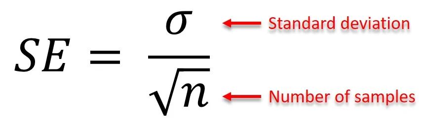
size of SE influenced by 3 factors

SD within the sample (larger SD = larger SE)

size of the sample (larger sample = sample mean closer to population mean)

proportion of the population covered by the sample (larger proportion covered in samples = lower variability of the means) - this has less influence on SE

confidence interval (CI)

how accurate an estimation of a population parameter will be

normally indicated as a % where the population mean lies within an upper and lower interval

use this to indicate the range we are pretty sure the population mean lies between 90, 95, 99% CIs

the larger the CI, the less precise the estimation of the population parameter

what would a 95% CI mean

a range of values that you can be 95% confident will contain the true mean of the population

what influences the size of CIs

variation

• low variation = smaller CI

• high variation = larger CI

sample size

• smaller sample = more variation = larger CI

• larger sample = less variation = smaller CI

calculating confidence intervals

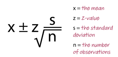
Z value

how many standard deviations a value is from the mean of a distribution

a measure of how many SDs the raw score is above/below the population mean (data that is recorded before going through statistical analysis)

based on a normal distribution

ranges 3 SDs above and below the mean

hypothesis testing steps

process of making inferences based on data from samples in a systematic way, to test ideas about the population

1) defining the null hypothesis

2) defining the alternative hypothesis

3) determining the significance level

4) calculating the p-value

5) reaching a conclusion

hypothesis testing 1) defining the null hypothesis

this assumes there is no difference between groups

nullifies the difference between sample means, by suggesting it is of no statistical significance

tests the possibility that any difference is just the result of sampling variation

hypothesis testing 2) defining the alternative hypothesis

predicts/states there is a relationship between the 2 variables studied

null hypothesis is assumed unless the difference between sample means is too big to believe the samples are the same (reject null hypothesis if differences become too big)

hypothesis testing 3) determining the significance level

typical level = 0.05 / 5%

known as the alpha

defines the probability that the null hypothesis will be rejected

similar outcomes reproduce 95% of potential replications

implies that in 5% of replications we will:

• observe an effect that isn’t real (type 1 error)

• fail to find an effect that does exist (type 2 error)

hypothesis testing 4) calculating the p-value

the probability value

how plausible is our data if there was actually no effect (null hypothesis true)

shows probability of an observed effect if the true (unknown) effect is null

between 0 (never) and 1 (always) probability

compare this against the significance level (alpha value)

p<alpha = significant

p>alpha = not significant

a p-value of 0.0125 means if the null hypothesis is true, the probability of obtaining results as/more extreme than those obtained is equal to 0.0125

if the p value is LESS THAN (<) alpha/significance level

reject null hypothesis

in favour of alternate hypothesis

results are statistically significant

we always say ‘reject (or fail to reject) null hypothesis’ when talking about significance, not ‘accept alternative hypothesis’

if the p value is GREATER THAN (>) alpha/significance level

fail to reject the null hypothesis - as this is evidence for the alternate hypothesis

results are NOT statistically significant

data is not inconsistent with null hypothesis

we don’t learn anything as evidence is inconclusive

if p-value is exactly 0.05, we still fail to reject null hypothesis

type 1 error

reject a true null hypothesis

rejecting it when should be accepting it

false positive

probability of making this error is represented by the significance level

can reduce risk by using a lower p-value (0.01 instead of 0.05)

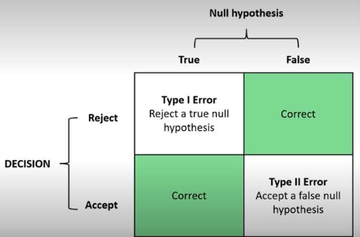
type 2 error

accept a false null hypothesis

accepting it when should be rejecting it

false negative

probability of making this error is know as beta

can reduce risk by making sure the sample size is large enough to detect a difference when one exists

regions of rejection

determined by the alpha level

known as critical region too

set of values for a test statistic that lead to the rejection of a null hypothesis

the term 1/2 tailed test refers to where these regions are

two-tailed test

non-directional

region where you reject the null hypothesis is on both tails of the curve

eg. alpha level of 0.05 - split between the 2 tails evenly, giving 2.5% to each tail (these are regions you reject null hypothesis)

research question would not specify the direct of effect (eg. difference, impact, affect)

one-tailed upper test

region where you reject the null hypothesis is on the right side/upper end of the curve

eg. alpha level of 0.05 - alpha is all at one end (not split evenly), giving 5% to the upper tail only (region to reject null hypothesis)

upper tail contains upper values in a distribution = higher numbers will appear here so research questions specify the direction of effect (eg. greater/more than, higher)

one-tailed lower test

region where you reject the null hypothesis is on the left side/lower end of the curve

eg. alpha level of 0.05 - alpha is all at one end (not split evenly), giving 5% to the lower tail only (region to reject null hypothesis)

lower tail contains lower values in a distribution = smaller numbers will appear here so research questions specify the direction of effect (eg. lower/less than, decrease)

quantitative research

develop research question and hypotheses using literature review

design study

determine analyses (need to know method, analysis depends on study design)

collect data

analyse data

interpret data

disseminate results

choosing an inferential test

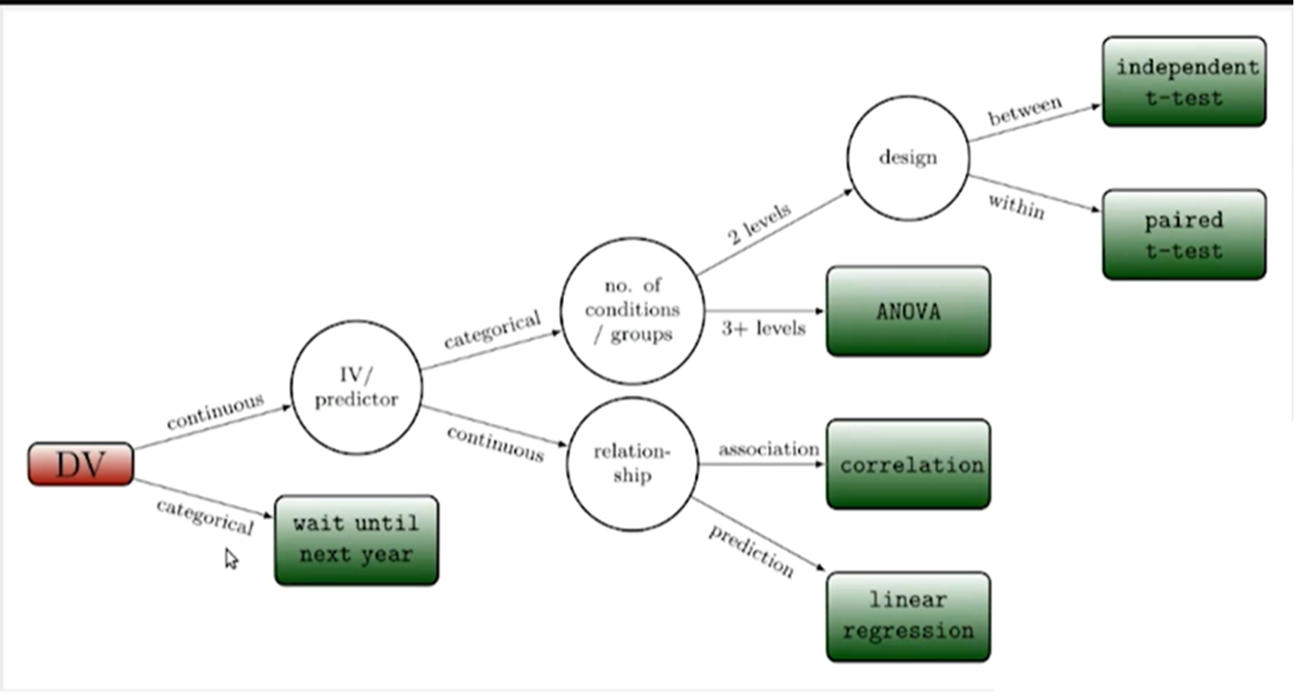
uni-variate data

1 variable

eg. asking 100 people their height and nothing else

summarising - mean and SD
visualising - histograms, box plots

understanding - results, normal distribution/skewness

can only answer simple questions

doesn’t help us understand why people act/think the way they do

bi-variate data

2 variables

eg. asking 100 people their height and weight

can be 2 continuous, 2 categorical or 1 of each

scatterplots

used with 2 continuous variables

a correlation used to measure strength of relationship between 2 variables

shows how much of the variance in 1 is explained by another

each point represents an observation

can see pattern, spread and orientation of the data

bigger sample size is better to reveal if relationship is real, but significant relationships aren’t the same as strong ones

interpreting scatterplots

shows how much of a relationship there is and the type

look at line of best fit, see how far spread out data points are from line, if there’s any anomalies

types of relationships:

• linear

• curvilinear

• exponential

linear relationships

straight line

as one variable changes, the other changes

rate of change remains constant

curvilinear relationships

as one variable changes, the other changes but only up to a certain point

after this point, there’s no relationship or direction of it changes

eg. Yerkes-Dodson

exponential relationships

as one variable changes, another changes exponentially

eg. world population

positive relationship

one variable increases, the other increases

negative relationship

one variable increases, other decreases

no relationship

scatterplot points don’t form a pattern

correlations quantify relationships

strength - how much of a relationship

significance - likelihood of finding the observed relationship in the sample, if there was no relationship in the population

variance explained by our model

line through all data points

line of best fit - smallest distance = bigger effect

models the correlation and relationship between variables

correlation

association between 2 continuous variables

Pearson’s estimates how much of the variance in one variable can be explained by another variable

Pearson’s correlation coefficient (r)

size of the effect = correlation coefficient (r) - between -1 and +1

squaring the correlation coefficient tells how much variance in the data is explained by the model - can convert to %

no relationship - r=0

moderate - r=0.5

perfect relationship - r=+1 or r=-1

linear regression

a modelling technique used to make predictions about an outcome variable, based on 1+ predictor variables (1 = simple linear regression)

establishes link/relationship between outcome and predictor variables

regression is the foundation to other types of regression analysis

tells us:

• strength of relationship between 2 continuous variables (so does correlations)

• statistical significance (so does correlations)

• how much one variable changes as another variable changes

• the value of one variable if the other variable was 0

• can predict a person’s score on a variable

includes effect size, slope and intercept

change in outcome variable (DV) for every unit increase in the predictor variable (IV)

• outcome y can be predicted as linear function of x

regression as a model

predictor variable (x) → outcome variable (y)

arrow points towards variable trying to be predicted

both continuous

still cannot infer causality

effect size - linear regression

shows the strength of relationship between 2 continuous variables

R² is a proportion of the variance explained by model (x100 to get %)

• how well does the model (regression line) represent the data

• strength of relationship (0-1)

modeled by how close our data points are to line of best fit

better the model, closer the points are to line of best fit

slope

beta (β)

shows how much one variable changes as another variable changes

essentially the line of best fit

intercept

a / constant (β₀)

where the line of best fit intersects the y-axis

the value of one variable (outcome) if the other variable (predictor) was 0

using regression for predictions

if value of x is known for a given participant, we can predict y

y = bx + a + error

y = (slope x x) + intercept + variance explained by other stuff

the error is taken off for predictions

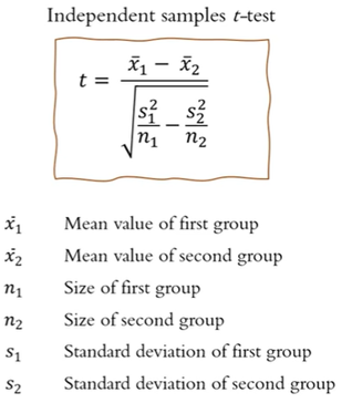
independent t-test

used to establish whether 2 means collected from independent samples differ significantly (difference between groups)

the null hypothesis is that the population means from the 2 unrelated groups are equal (most the time we reject the null and accept alternative - means are NOT equal)

the difference between the means of 2 independent groups

t = difference between groups / variance within groups

more extreme t value (>2) indicates less overlap between groups

features of independent t-test datasets

1 independent variable with 2 independent groups (between groups design)

1 dependent variable measured using continuous and normally distributed data

what do independent t-tests take into account

the mean difference between samples

variance of scores

sample size

t-statistic

produced from a t-test

the ratio of the mean difference between the 2 groups and the variation in the sampled data

uses the mean difference between samples, sample size and variance of scores

paired samples t-test

repeated measures - compare samples where each group participated in both conditions

data is collected from the same participant for both sets of observations (paired observations)

used to establish whether the mean difference between 2 sets of observations is 0

average size of change for each participant

t = score change / variance of that change

degrees of freedom = number of pairs - 1

features of paired samples t-test datasets

1 independent variable with 2 dependent groups (within groups design)

1 dependent variable measured using continuous and normally distributed data

one-way ANOVA

analysis of variance

tests whether there are statistically significant differences between 3+ samples (between-groups design)

one-way is specifically for samples that are independent groups

tests the null hypothesis that the samples in all groups are drawn from populations with the same mean values (and there is no significant difference between them)

accounts for both the variance between groups and within groups

features of a one-way ANOVA

1 independent variable with 3+ conditions/levels/groups

1 dependent variable measured using continuous and normally distributed data

ANOVA terms

one-way = 1 independent variable

factorial = multiple independent variables

ANCOVA = covariate (control variable)

MANOVA = multiple dependent variables

factors = independent variables

effects = quantitative measure indicating the difference between levels

why is multiple testing/comparisons a problem

if we adopt alpha level of 0.05 and assume the null hypothesis is true, then 5% of the statistical tests would show a significant difference

the more tests we run, the greater likelihood that at least 1 of those tests will be significant by chance (type 1 error - false positive)

when multiple testing issues arise

looking for differences amongst groups on a number of outcome measures

analysing data before data collection has finished, then re-analysing it at end of collection (this violation often used to see whether more data needs to be collected to reach significance)

unplanned analyses (conducting additional ones to try to find something of interest)

how to solve multiple testing issues

avoid over-testing (plan analyses in advance)

use appropriate tests

when multiple tests are run, adjust the alpha threshold

test statistic

a value that is calculated when conducting a statistical test of a hypothesis

shows how closely observed sample data matches the distribution expected under the null hypothesis of that statistical test

used to calculate the p-value of results

eg. t-test produces t statistic, ANOVA produces f statistic

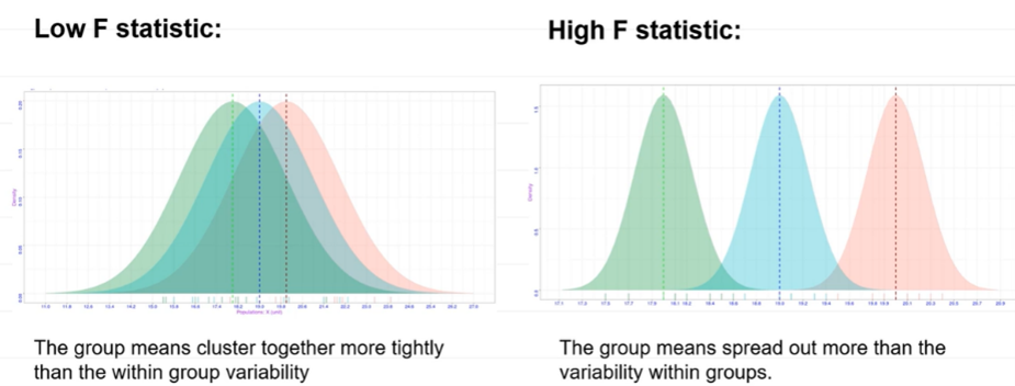
the F statistic

an ANOVA produces this test statistic

a ratio of 2 variances (mean squares)

how much more variability in the data is due to differences between conditions/groups, as opposed to the normal variability

this along with degrees of freedom are used to calculate the p-value

if variants of the between groups is similar to the variants of the within groups, F statistic will be near 1

calculation: variance between groups/variance within groups