PHYS 1011: Chapter 1 and 2

Physics

Concerned with describing the interactions of energy, matter, space, and time. Interested in the fundamental mechanisms that underlie every phenomenon.

• Structured by natural law.

Model

Representation of something that is often too difficult to display directly.

• Helps physicists analyze a scenario and do calculations, or represent a situation with a simulation.

Theory

A testable explanation for patterns in nature, supported by scientific evidence and verified multiple times.

• Describes all aspects of an applicable system.

• Less concise

Law

Describes a generalized pattern in nature that is supported by scientific evidence and repeated experiments.

• Concise and a very general rule for phenomena in nature.

• Single action

Scientific Method

Begins with an observation that is researched, then develops a hypothesis, which they test through an experiment. They analyze the results and draw conclusions.

Classical Physics

Developed from the Renaissance to the end of the 19th century.

• Developed into modern physics.

• Gives an accurate description of the universe and is the basis for understanding modern physics.

Modern Physics

• Relativity: used when an object is traveling at speeds >1% of the speed of light in a strong gravitational field.

• Quantum Mechanics: Applies to objects smaller than can be seen with a microscope.

Physical Quantity

Defined by specifying how it is measured of by stating how it is calculated from other measurements.

SI Units

• Length = meter (m)

• Mass = kilogram (kg)

• Time = seconds (s)

Fundamental Units

Describe measurements by how they were measured.

• SI Units

Orders of Magnitude

Each power of 10 is a different order of magnitude; numbers that can be expressed by the same power of 10 are the same order of magnitude.

• Ex: 800 = 8 × 10² and 450 = 4.5 × 10²

Conversion Factors

A ratio expresses how many of one unit are equal to another unit.

• Orient into a fraction with the unit needed to be canceled on the bottom

Accuracy

How close a measurement is to the correct value

Precision

How close repeated measurements are to each other

• Clump of points, rather than a bullseye

Uncertianty

A quantitative measure of how much your measured values deviate from the expected value.

• There is more uncertainty if accuracy and precision are low

• Denoted as A ± unc_A

• Contributing Factors: limitations of a measuring device, skill of the measurer, irregularities in the measured object, and other factors affecting the outcome.

Percent Uncertainty (%unc)

%unc = (unc_A / A) x 100

Adding Percent Uncertainties

When adding two measured values, just add their uncertainty quantities together to find the final solution.

• Same for subtraction.

Multiplying Percent Uncertainties

When multiplying two measured values, find their individual %unc and add them together to find the total %unc.

• To convert back to a value, multiply the percent by the final product.

• Same for division.

Significant Figures - Measuring

The last digit written down from a measurement is the first digit with some uncertainty.

• The known digits and one estimated digit, which may be a “.0” if necessary. The precision on a measuring device is dictated by the number of markings and how fine they are.

• Exceeds the specificity of the tick marks.

• The more significant figures → the more precise

Significant Figures

The digits in a measurement, including the uncertain last digit.

• Zeros: captive and trailing zeros (when a decimal is present) are always significant

Sig Figs - Calculations

When performing calculations, the result can never be more precise than the measurements upon which it is based.

Rules for Counting Sig Figs

1. Nonzero integers are always significant

2. Zeros: 3 cases…

(a) Zeros between two nonzero integers are always significant

(b) Zeros that precede nonzero integers are never significant

(c) Zeros at the right end of a number are significant only if the number contains a decimal point

3. Exact numbers have an infinite number of significant figures

Rounding Sig Figs

• Adding/Subtracting: the least number of decimal places

• Multiplying/Dividing: the fewest number of significant figures

  • Average: don’t incorporate the denominators’ sig figs into the answer

Uncertainty Types

• Systematic: consistently causes the value to be too large or too small.

• Random: variations that occur unpredictably.

• Causes distributions with the center being the measurement and the deviations being the uncertainty.

Estimating Uncertianty

Use significant figure rules for measurement and add an applicable range.

Average Deviation

Take the average of all of your measurements, then the absolute value of the difference of each from the average, then find the average of the deviations.

Estimating Uncertainty

Use the largest possible uncertainty the calculation could yield, which will always overestimate the uncertainty of the calculations.

Precision Calculation

(unc./measurment) x 100%

Position

Where an object is at a particular time

• Relative to a convenient reference frame, which is usually stationary objects

Displacement

When an object moves relative to a reference frame

• ∆x = x_final - x_initial = x_f - x_i

• SI unit = meters (m)

• Has a direction (±) as well as a magnitude

  • Positive = right or up

  • Negative = down or left

Distance

The magnitude/size of the displacement between two positions

• Not the same as distance travelled

• Has no direction

Distance Travelled

The total length of the path traveled between two positions.

Vector

Any quantity with both a magnitude and direction (+ or -)

• Velocity and distance

• Represented graphically with an arrow, which has the length of the magnitude and points in the same direction

Scalar

Any quantity that has a magnitude but no direction.

• Ex: magnitude, negative degrees C

Coordinate System for 1D Motion

• +y = up (N)

• -y = down (S)

• +x = right (W)

• -x = left (E)

Time

Change/the interval over which a physical quantity changes

• Elapsed Time: how long it takes ___ to ___ …

Average Velocity

Displacement (change in position) divided by the time of travel.

• v = ∆x/∆t = x_f - x₀ / t_f - t₀

• Vector quantity

• The magnitude of the average velocity is smaller than or equal to the average speed

Instantaneous Velocity (v)

The average velocity at a specific instant in time (instantaneous, small time interval)

• Only a magnitude usually

• The slope of the curve in a position vs. time graph at time t

Instantaneous Speed

The distance traveled divided by the elapsed time

• Magnitude of the instantaneous velocity

Average Acceleration

The rate at which velocity changes

• a = ∆v/∆t

• SI unit = m/s² (by how much the velocity changes every second)

• An acceleration is when velocity changes in magnitude, direction, or both.

• Vector is in the same direction as the ∆v

Deceleration

When an object slows down, and it’s acceleration is opposite to its motion

• Slows down = opposite vector of velocity

• Occurs when the acceleration is opposite in direction to the velocity

Instantaneous Acceleration (a)

Acceleration at a specific instant in time (infinitesimally small interval of time)

Notions

∆t = t, ∆x = x - x₀, and ∆v = v - v₀

• Where the initial values = 0

• Also assume acceleration is constant (ā = a = constant)

Velocity - Constant Acceleration

v = v₀ + v / 2

Displacement - Velocity

Have a linear relationship, where it is determined by velocity multiplied by time

• x = x₀ + vt

Displacement When Velocity isn’t Constant

x = x₀ + v₀t + ½ at²

• Displacement depends on the square of elapsed time when acceleration isn’t θ

Final Velocity - Velocity isn’t Constant

v² = v²₀ + 2a (x - x₀) (constant)

Problem Solving Steps

1. Examine the situation to determine which physical principles are involved; draw a simple sketch (note the positive direction)

2. Make a list of what is given or can be inferred

3. Identify exactly what needs to be determined in the problem (unknown)

4. Find an equation or set of equations that can help solve the problem, ideally ones with only one unknown variable

5. Substitute the knowns along with their units into the appropriate equation, and get numerical solutions with units

6. Check to see if the answer is reasonable

Gravity

If air resistance and friction are negligible then in a given location, all objects fall toward the center of the earth with the same constant acceleration, independent of their mass

Free - Fall

An object falling without air resistance or friction

Acceleration due to Gravity

The acceleration of free-falling objects

• g = 9.8 m/s

Kinematic Equations for Free-falls Where a = -G

• v = v₀ - gt

• y = y₀ + v₀ + ½ gt²

• v² = v²₀ - 2g (y - y₀)

Graphs - Axis

The horizontal axis (x) represents the independent variable, and the vertical axis (y) represents the dependent variable

• y = mx +b

  • m = slope

  • b = y-int

Graph of Position vs. Time (a = 0, v is constant)

Time is independent, and position is dependent

• x = x₀ + vt

• slope (m) = velocity

Graphs of Motion When a is constant, but ≠ 0

Velocity is constant, and acceleration is a y = # graph

• position vs. time is a curve

• slope of velocity vs. t = acceleration ( v = v₀ + at)

Trajectory ≠ Displacement

A displacement vector starts at the object’s initial position and ends at its final position, not taking into account any of the motion in between. The trajectory depends on the motion in between.

• Motion: change of an object’s position or orientation over time

• Trajectory: Path along which an object moves

Particle Motion Model

An object is at a single point; over the same interval of time passing, the model depicts the motion of the object at those points as successive dots.

Round Trip Displacement

0

Vector

Notation: A

Magnitude: |A|

Operations With Velocity

• Addition: A + B = B + A or (A + B) + C = A + (B + C)

• Subtraction: A - B = A + (-B)

Position vs. Time Graph

Use the particle model to make a continuous curve, where the position is the y-axis.

• Velocity = the slope

Velocity Vector

• v₁ = v₁j, magnitude |v₁| = v₁

• v₂ = -v₂j, magnitude |v₂| = v₂

Velocity vs. Time Graph

A graph where the y-axis represents velocity, and the graph has horizontal line segments when velocity is constant, and dotted vertical increases between velocity changes.

• Velocity → Position: ∆x = velocity x ∆t

  • Use the constant velocity segments as slopes between positions (x)

Uniform Motion

Constant motion at a constant velocity (no acceleration), with a straight-line motion where there are equal displacements during successive equal time intervals.

• Straight-line slope (time vs. position)

Equation of Uniform Motion

x_f = x_i + v_x∆t (x is position)

Displacement - Curve

The displacement ∆x is equal to the area under the velocity graph during an interval ∆t

Displacement Notes

It is the difference between two coordinates so it doesn’t depend on the origin

From Velocity to Acceleration

• Constant increasing positive slope in a velocity vs. time graph → horizontal positive line

  • Same for constant deceleration, but the horizontal line is -y on the acceleration graph

• Slope of velocity is constant, meaning that the horizontal acceleration segment = 0

Sign of Acceleration

v_x is accelerating

• to the right = + slope

• to the left = - slope

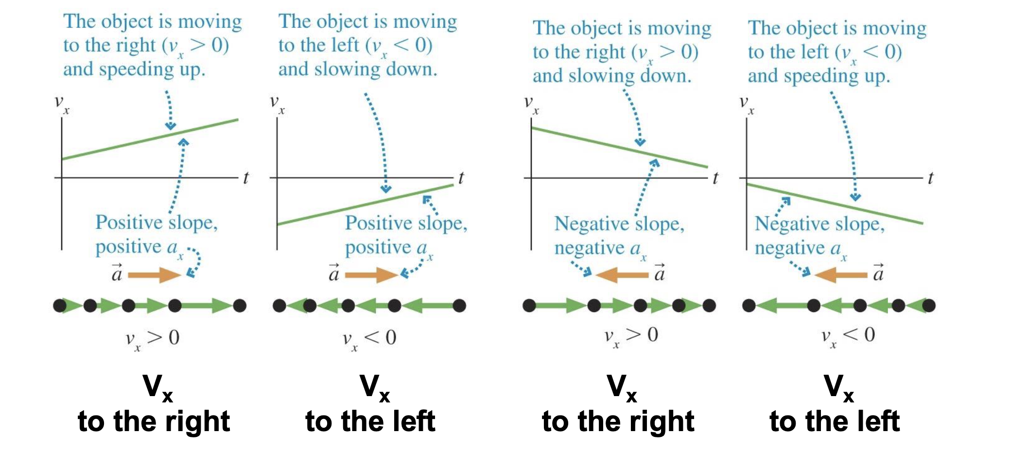
Negative Acceleration

Acceleration in the negative direction (v₁ = - )

• Magnitude matters

Acceleration Equations

Motion at Constant Velocity vs. Constant Acceleration

a) Constant velocity: position = + slope, velocity = horizontal, acceleration = 0

b) Constant Acceleration: position = quadratic, velocity = + slope, acceleration = horizontal

Velocity vs. Time - Displacement

Calculate the area under the desired segment to determine the displacement in meters

• Go all the way down to the x-axis

Free Fall - Notes

Acceleration is constant (A = B = C = D = E) because different lb weights hit the ground at the same time, and an arrow’s path has the same acceleration at all points.

• “Drop” = initial velocity of zero and decelerates as it moves up

Position vs. Time - Velocity Slope on a Curve

Draw a straight line at the specific point

• Parallel = same velocity

• Tangent line