Applied econometrics lectures 11-14 - Panel data

Panel data defenition

repeated observations over time for the same individual

Pooled cross sectional data

•       Two or more similar cross-sectional datasets, each relating to a different time period 

•       Variables contained in each cross section are the same

•       Samples of observations are not the same (may overlap)

pooled vs panel

The repetition of going back to the same people is what makes the data panel - Contains a time series for each cross-sectional unit

• Pooled cross section datasets the samples in any two years are independent

• Panel datasets the samples in any two years are not independent, they are the same

Why is panel data the most powerful

allows us to control for unobserved (time-invariant) heterogeneity

Why panel data violates OLS

the error terms relating to some pairs of observations may be correlated with one another

But we can use it to our advantage

what happens if we ignore the time dimension with panel data

when estimating you might not be estimating what you think due to the non-independence

We can run regressions separately to combat this

Possible problem with running regressions separately

Omitted variable bias (OVB) – zero conditional mean doesn’t hold

The effect of all those other variables is currently in the error term making it difficult to get an accurate estimate of the relationship we are interested in → high p values

Solutions to OVB with panel data

•Add more explanatory variables

•Focus on the second year and add a lagged dependent variable

•Pool across the years so we have more observations => more power

• does this fix the independence issue? - NO

•Exploit the panel and have a think explicitly about the structure of the errors

Error term as 2 parts

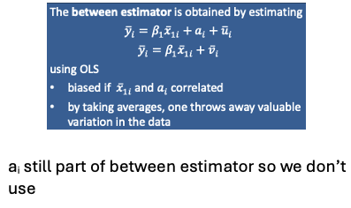
Fixed effect - a_i Captures all unobserved, constant factors that affect y

• Geographical factors + Institutional factors

Idiosyncratic effect - U_it Captures all other unobserved factors

How to estimate the models with split errors

Pooled OLS

First differences

Pooled OLS with split errors

Assume a_i & U_it uncorrelated with x_it → can use OLS as Zero conditional mean not broken

Combine error terms back together - a_i + U_it = v_it E(v_it | x_it) = 0

If they are correlated then we get biased estimators

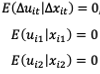
First differences model

When we use first differences, a_i drops out as its time invariant - same in both periods

First differences and OLS

After differencing, we no longer have 2 sets of restriction to estimate

We can use OLS to get unbiased estimates so long as:

No worse off than before - still have to worry about this

First differences constant / intercept

In the first difference model, we don't have anything that tells you what would be the average level of crime if there was zero unemployment.

Our intercept tells you what was the average change

First differences if x_it varies little over time

First differencing eliminates time-invariant error + reduce OVB + increase accuracy of estimates & power

When X varies little then OLS estimators are extremely unstable as they will have huge standard errors - no relationship evident

Downsides of Panel data

Data availability & quality

Econometrically

Downsides of Panel data - Data availability and quality:

• Panel data is costly to collect

  • tracking people/households/firms for a second/ third/fourth … interview is time-consuming and even more costly when using repeat people

• sample attrition: some people/ included in earlier rounds are not found in later rounds

  • Problematic if non-random

    • i.e. if the likelihood of finding them is systematically related to something we are interested in, e.g., better performing firms are more likely to be findable second time around

  • Over time, the sample may become less representative

    • Under-samples migrants in countries who recently have high immigration if survey started before high immigration

• Much less of a problem with administrative data (very popular in modern research)

  • No attrition

Downsides of panel data - econometrically

Differencing does not help if the variables of interest do not change or change very little over time

– If they don’t change at all: you can’t estimate anything

– If they change little: you might estimate something off of noise

The potential for omitted variable bias still exists

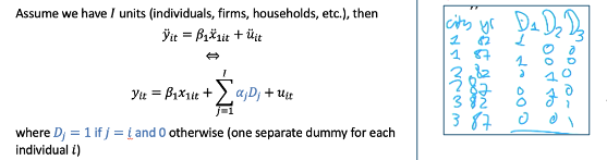
Extending the model to include t > 2

Add dummy variable for each year - captures avg change between years in the panel across all respondents

Extending the model - first differences

We can still use first differences when t > 2 as it still eliminates a_i

However we need to worry about serial correlation

• if u_it follow AR(1) then change in u_it are serially correlated

• If u_it are uncorrelated with constant variance, the correlation between the changes in t is -0.5

We need to adress heteroscedasticity

Fixed effect transformation

One of other way to eliminate time-invariant unobservables

average of a_i = a_i (constant)

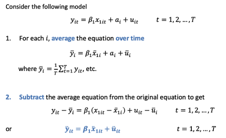
Fixed effects estimator

When we apply fixed effects / within transformation to OLS we get our estimators

We rely on differences within each sample unit (not sample) to idnetify the relationship (variation between y_it & x_i within i)

we still need E( ̈u_it | ̈x_it) = 0 across all t to get unbiased

Between estimator

Fixed effects estimator and se(^β₁)

To get unbiased estimates we need to adress heteroscedasticity

We also need u_it to be serially uncorrelated

Fixed effects estimation - Degrees of freedom

df = NT - N - k

i = 1, 2, … , N t = 1, 2, … , T

-k not (-k -1) as we are estimating a constant

-N as we have to estimate the means

(-N -k) as we are estimating N constants + we lose N when we take an avg

When are Fixed effects and First difference equal

FE = FD when T = 2

Fixed effects and Least squares dummy variable model

FE = LSDV

Within transformation can be obtained by including dummies for all i

Fixed effects when there are fixed variables

FE estimation cant estimate fixed variables, or variables with a time trend (becomes spurious for each individual)

We split the data into what varies and what doesn’t

• if var fixed but with time trend we remove i & t. but add t as part of the coefficient

• If just fixed then remove t

We include dummies to see effect every year

a_i & fixed var drop out when we apply FE transformation

• fixed with time trend fall out as constant for each individual

Time invariant regressors and stata omitting

Stata omits the time invariant regressors (‘omitted due to collinearity) as it thinks it’s a constant

Not a problem if variable doesn’t vary – but if it varies very little then stata will still give an estimate and it will affect everything else

Time invariant regressors and interaction terms

in order to get round stata omitting the variables that only vary in i, we include an interaction term with the time dummy variable

now it varies in i and in t

stata estimate now shows what the returns are of that var in every year

In the example the estimate got bigger for every year of educ → return to educ increase over time the longer in the L market

Random effects model conditions needed

If a_i is uncorrelated with x_jit in all time periods

• then we don’t need to get rid of it to get unbiased estimates → no OVB

RE model and composite errors

We combine a_i & u_it back together → v_it

However the composite error will be serially correlated with i as they all share a_i → OLS biased

Therefore we use GLS

composite error

v_it = a_i + u_it

Generalised Least Squares (GLS)

As long as we have large N relative to T we can use GLS - data on lots of units over few years

GLS involves partially demeaning our dependent and explanatory variables & our errors

GLS post partial demeaning

Partially demeaning - takes a proportion of the mean away (proportion = λ)

FE completely demeans

λ equation - measure of relative importance of varianve in idiosyncratic error compared to unobserved fixed effect

partially demeaned time-invariant explanatory variables

remains in the model (doesn’t = 0)

Can be estimated

To get unbiased estimates we need to assume all explanatory variables are uncorrelated with u_it & a_i in every t

σ_a² & t effects on dataset

As they increase:

• The more important the variance in time invariant unobservable

  • The larger we want λ to be

• The closer λ is to 1 - The more of the time invariant part of error we take away

  • to get rid of serial correlation in composite error

λ at the extremes

λ = 1 → FE transformation

λ = 0 → OLS pooled sampled

• y bar = 0

  • y_it - y bar = y_it

RE vs FE efficient

RE is more efficient

• gives better confidence estimates + better inference

Makes better use of the data

• demeaning in FE loses some variation (more than needed)

However if all x_it are not uncorrelated with a_i → FE is only choice

Why do we compare RE & FE

By comparing FE & RE we can draw inferences about likely biases

What Hausman test tests for

We can test cov( x_ij , a_i ) = 0 by comparing estimated coefficients on time-varying x in FE & RE model

If a_i is uncorrelated with Xs then FE is not efficient as inflated SE

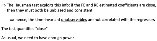
Hausman test null

H₀ : a_i uncorrelated with included regressors

• both FE & RE unbiased + consistent

• Difference in coefficients not systematic

H₁ : a_i correlated with included regressors

• RE inconsistent

When do pooled 1st difference OLS and within estimator yield identical results

When T = 2