L5_Optimizers and Learning Rates

Flashcards on optimizers, loss functions, and learning rates in deep learning.

What is a Loss Function?

A differentiable measure (L >= 0) of prediction quality, bounded below. It quantifies how well a model's predictions match the actual values. It needs to be differentiable so we know how to adjust the models, and bounded below so we have a direction we want to head, which is to minimize! Analogy: Like measuring the distance between a map (prediction) and the actual terrain (reality). We want this distance to be as small as possible, ensuring our map accurately represents the real world.

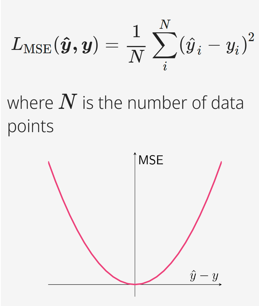
What is Mean Squared Error (MSE) Loss?

LMSE(y^, y) = (1/N) \* ∑(y^i - yi)^2 , used for regression tasks. It calculates the average of the squares of the errors between predicted and actual values. The squaring emphasizes larger errors and ensures the loss is always positive, preventing errors from canceling each other out. Analogy: Measures the average squared 'miss' distance in a series of shots. Larger misses are penalized more, pushing the aim to become more accurate.

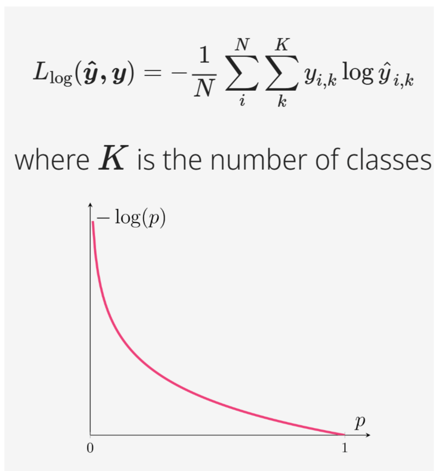
What is Cross-Entropy Loss (Log Loss)?

Llog(y^, y) = -∑∑ yi,k \* log(y^i,k), used for classification tasks. It quantifies the difference between two probability distributions (predicted and actual). The closer the predicted probability is to the actual value, the lower the loss, indicating a better model's prediction. Analogy: It's like measuring how surprised you are when the actual outcome differs from your predicted probabilities. Lower surprise means better prediction.

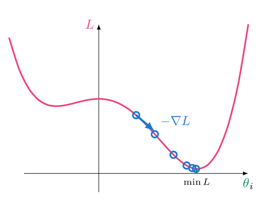
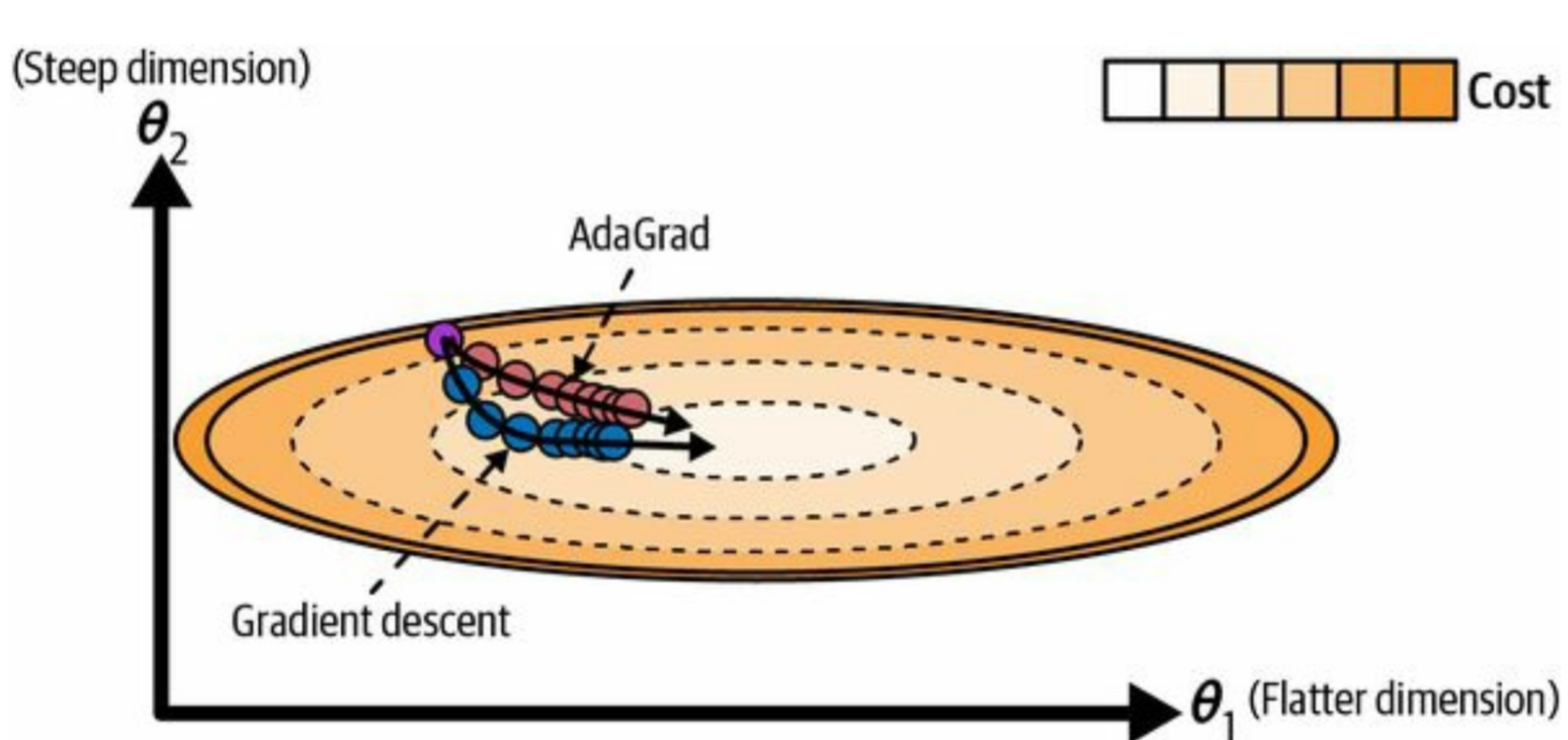
What is Gradient Descent?

θn+1 = θn − η∇L, where η is the learning rate. It's an iterative optimization algorithm to find the minimum of a function by taking steps proportional to the negative of the gradient of the function at the current point, guiding the model towards optimal parameters. Analogy: Like rolling a ball down a hill; it takes steps in the direction of the steepest descent, seeking the lowest point in the landscape.

What is Momentum Optimization?

Keeps track of past gradients to improve gradient descent. It adds a fraction of the previous update to the current update, smoothing the optimization process and helping accelerate convergence in the relevant direction, preventing oscillations and speeding up learning. Analogy: Like a ball rolling down a hill gains momentum, helping it overcome small bumps and maintain direction.

What is the Momentum update rule?

θn+1 = βmn−1 − η∇L(θn), where β is the momentum. The parameter update considers a fraction of the previous update vector. Incorporates historical gradients into the current update direction, stabilizing the learning process. Analogy: Builds inertia into the gradient descent process, allowing it to smoothly navigate the error surface.

What is Momentum?

A hyperparameter in momentum optimization that controls the amount of friction (β ∈ [0, 1]). The closer to 1, the more information to retain, allowing the optimization to maintain its direction. Analogy: The higher the momentum, the less friction the ball experiences rolling down the hill, maintaining its speed and path.

What is Nesterov Accelerated Gradient?

Compute the gradient slightly ahead when using momentum. It evaluates the gradient at the 'anticipated' future position to make corrections before actually getting there, improving stability and convergence. Analogy: Instead of blindly following the current gradient (like in standard momentum), NAG looks ahead in the direction where momentum is carrying us to correct its course, anticipating changes in terrain.

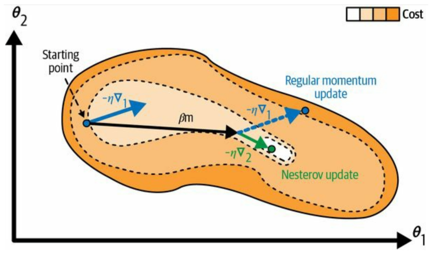
What is Nesterov accelerated gradient update?

mn = βmn−1 − η∇L(θn + βmn−1). The gradient is evaluated at the 'anticipated' future position. This adjusts the gradient calculation to account for the momentum, fine-tuning the optimization process. Analogy: Corrects trajectory before getting there, anticipating and adjusting for future movements.

What is AdaGrad (Adaptive Gradient)?

It introduces an adaptive learning rate, adjusted independently for different parameters by adjusting by the sum of all past gradients. It adapts the learning rate to each parameter, giving larger updates to infrequent and smaller updates to frequent parameters, optimizing each feature's learning rate. Analogy: Like having individual volume knobs for each instrument in an orchestra, automatically adjusting to balance the sound and fine-tune each instrument's contribution.

What is RMSProp (Root Mean Square Propagation)?

Optimization algorithm, Improves on AdaGrad by exponentially scaling down old gradients. It addresses AdaGrad's diminishing learning rates by discounting the influence of very early gradients, allowing for continued learning. Analogy: Only considers the recent gradients like focusing on recent traffic conditions, adapting to the most relevant information for current optimization.

What is Adam (Adaptive Moment Estimation)?

Momentum + RMSProp + some technical details. It computes adaptive learning rates for each parameter, incorporating both momentum and scaling of gradients. It's computationally efficient and well-suited for problems with large parameter spaces, combining the strengths of both techniques. Analogy: Like a car with both acceleration (momentum) and traction control (RMSProp), providing smooth and efficient movement.

What is AdaMax?

Scale the past gradients differently. A variant of Adam that uses infinity norm. Instead of using the squared gradients directly, it normalizes with the maximum of the past gradients, providing more stable updates. Analogy: Consider the absolute largest past gradients, using extreme values to normalize learning.

What is Nadam?

Add Nesterov momentum. It combines Adam with Nesterov Accelerated Gradient for faster convergence, providing a more efficient and stable optimization process. Analogy: Combining both acceleration and pre-emptive correction, enhancing the optimization's performance.

What is AdamW?

Add L2 regularization (aka weight decay). It decouples weight decay from the gradient-based optimization step. It helps prevent overfitting by penalizing large weights, promoting simpler models and better generalization. Analogy: Add stabilizing regularization separately than loss, preventing the model from becoming too complex.

What is the Learning Rate?

Affects training progress. Determines the step size during optimization. If too high might overshoot, if too low might take too long, impacting the model's ability to converge. Analogy: Like adjusting the stride length during walking. Too large and you might stumble; too small and you'll take forever to reach the destination.

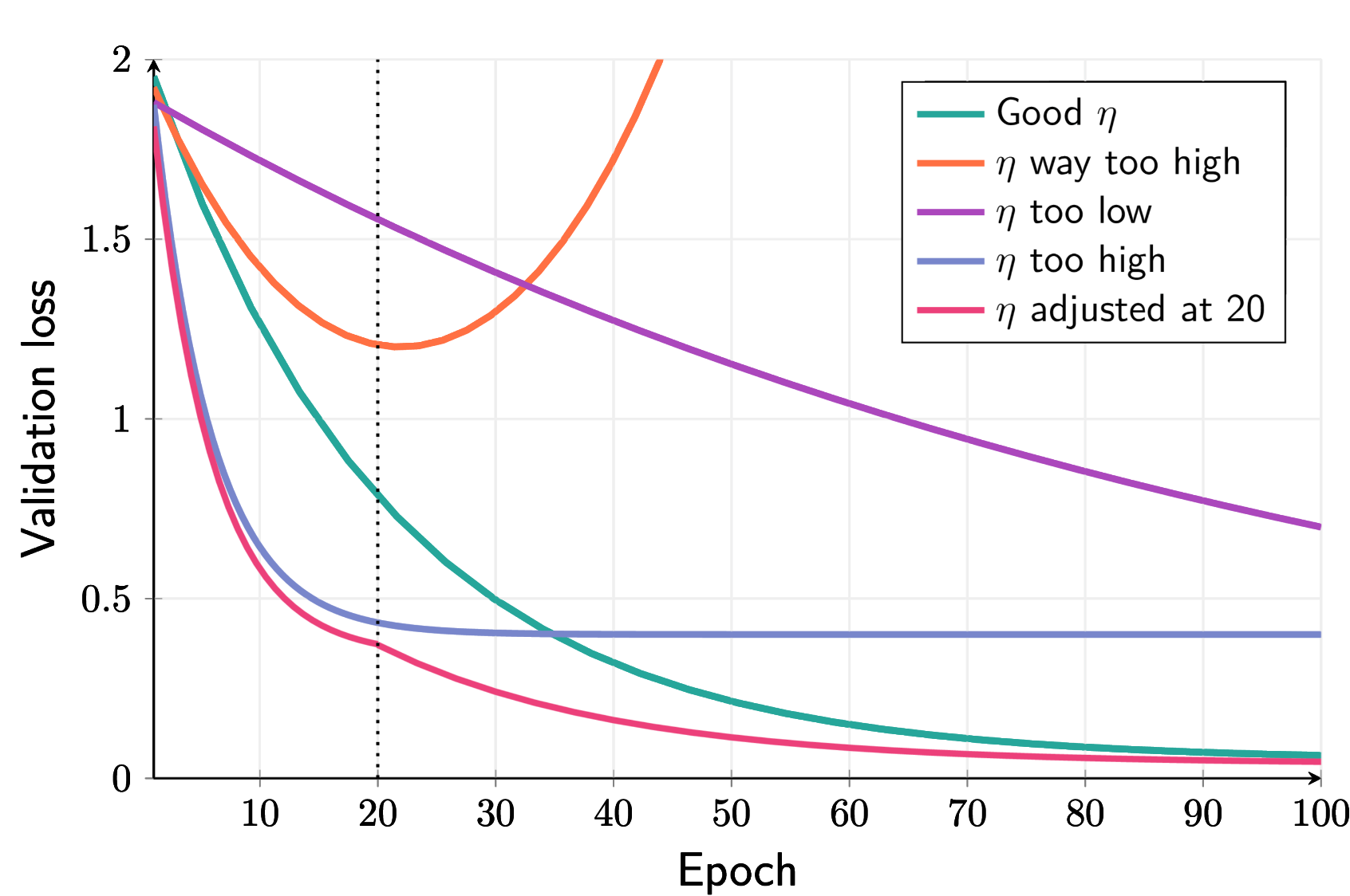
What is Learning Rate Scheduling?

Reduce learning rate when learning stops. This could improve convergence as a result, allowing the model to fine-tune its parameters more effectively. Analogy: Slowing down as you approach the destination, allowing for more precise adjustments.

What is Exponential Decay?

Gradually reduce η for each step. A common method of learning rate scheduling, reducing the learning rate over time. Analogy: Gradually reducing throttle, allowing for smoother control and adjustments as the model converges.