Equity 4: Financial Models

Three major categories of equity valuation models

(1) Present value models (a.k.a. discounted cash flow models) — intrinsic value as the PV of future benefits, defined as dividends (dividend discount models) or free cash flow to equity. (2) Multiplier models (a.k.a. market multiple models) — value from a price multiple (e.g., P/E, P/S) applied to a fundamental like earnings or sales, or an enterprise value multiple (EV/EBITDA, EV/revenue), where EV = total market value minus cash/short-term investments; equity value can be backed out of EV by subtracting liabilities and preferred shares. (3) Asset-based valuation models — value of equity = estimated value of assets minus liabilities and preferred shares, usually by adjusting the book (carrying) value of assets/liabilities to market value.

Dividends: key background facts for the DDM

Regular cash dividends are paid on a known schedule (quarterly in US/Canada, semiannually in Europe/Japan, annually in China, etc.); extra/special dividends are one-off, common in cyclical or restructuring companies. Dividends aren't a legal obligation until declared by the board. Stock dividends (bonus issues), stock splits, and reverse stock splits have no economic effect on firm or shareholder value (just divide the same "pie" into more/fewer pieces), so they're not relevant for valuation. Share repurchases (buybacks) are viewed as economically equivalent to paying an equal-value cash dividend; reasons include signaling undervaluation, flexibility in timing/amount, tax efficiency, and absorbing dilution from employee stock options. Dividend chronology: declaration date → ex-dividend date (first date a share trades without the dividend) → holder-of-record date (linked to the settlement cycle) → payment/payable date.

Free cash flow to equity (FCFE)

Free cash flow to equity (FCFE) model vs. the DDM\FCFE = CFO − FCInv + Net borrowing. CFO (cash flow from operations) = net income + non-cash expenses − investment in working capital; FCInv (fixed capital investment, often proxied by reported capex) is subtracted because it isn't available for distribution to shareholders, while net borrowing is added back since it is. Many analysts use FCFE instead of the DDM because FCFE reflects a company's dividend-paying capacity rather than the dividends it actually chooses to pay, which they see as the more fundamentally sound basis for valuation. FCFE is also the practical choice for non-dividend-paying stocks, since a DDM requires predicting the timing/amount of a first dividend and all dividend growth thereafter — often very difficult to do accurately when there's no dividend history to anchor on. FCFE valuation otherwise parallels the DDM: V₀ = Σ FCFEₜ/(1+r)ᵗ.

CAPM for the required rate of return

Required return on share i = risk-free rate + Betaᵢ × (market risk premium), where beta measures non-diversifiable risk and the market risk premium is the market's expected return in excess of the risk-free rate. Even when analysts agree CAPM is appropriate, differing inputs mean there's no single correct answer; alternatives include adding a judgment-based risk premium to a government bond yield, adding a premium to the company's own bond yield, or using a rate set by firm policy.

General dividend discount model (DDM)

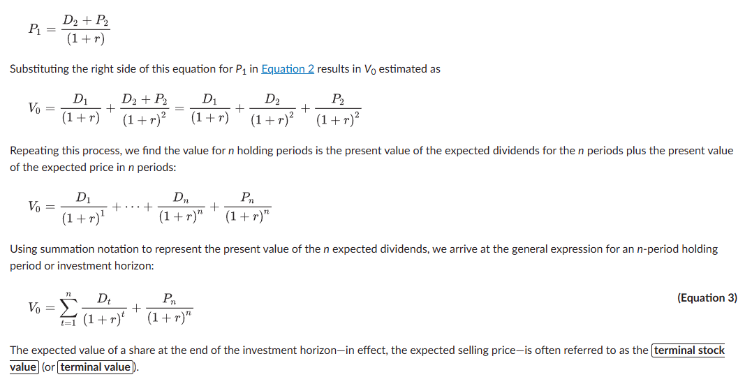
V₀ = Σ Dₜ/(1+r)ᵗ. V₀ = value of a share today, Dₜ = expected dividend in year t (paid at year-end), r = required rate of return. Holds regardless of the investor's actual holding period: for a 1-year holder, V₀ = D₁/(1+r) + P₁/(1+r), where the future price P₁ = (D₂+P₂)/(1+r) — substituting forward shows value depends directly on dividends received before a sale and indirectly on later dividends via the sale price. General n-period form: V₀ = Σ Dₜ/(1+r)ᵗ + Pₙ/(1+r)ⁿ, where Pₙ is the "terminal value" — the expected share price at the end of the horizon.

Perpetual preferred stock valuation

V₀ = D₀/r — the present value of a perpetuity. Applies to a non-callable, non-convertible perpetual preferred share paying a level dividend D with a constant required rate of return r. Preferred stock itself is a generally non-voting equity class with priority over common stock for dividends and liquidation proceeds; it may be perpetual or have a stated maturity (at which par value is paid), and may be callable or convertible.

Preferred stock valuation with a maturity date

V₀ = Σ Dₜ/(1+r)ᵗ + F/(1+r)ⁿ — same structure as the finite-horizon DDM but using the preferred's par value F in place of a terminal stock price. Most precise when n, r, and D match the actual payment schedule (e.g., semiannual dividends use a semiannual n, r, and D), just as with bond valuation. A call option held by the issuer reduces the preferred's value to the investor (issuer redeems only when favorable to itself); a retraction (put) option held by the investor increases its value (investor exercises only when favorable to itself). This formula can also approximate the value of callable/retractable preferred stock.

Gordon (constant) growth model

V₀ = Σ [D₀(1+g)ᵗ]/(1+r)ᵗ, which (when r > g) reduces to V₀ = D₀(1+g)/(r−g) = D₁/(r−g) — note the numerator is D₁, not D₀. Values equity as the present value of a growing perpetuity (reduces to V₀ = D₀/r if g = 0). Best suited to dividend-paying companies that are relatively insensitive to the business cycle and in a mature growth phase, especially with a history of raising the dividend at a stable rate.

Sustainable growth rate

g = b × ROE, where b = earnings retention rate = (1 − dividend payout ratio) and ROE = return on equity. One of several ways analysts estimate the long-term dividend growth rate for the Gordon model (others: historical dividend/earnings growth, industry median growth rate).

Assumptions of the Gordon growth model

(1) Dividends are the correct valuation metric; (2) the dividend growth rate is perpetual and never changes; (3) the required rate of return is also constant over time; (4) the growth rate is strictly less than the required rate of return.

Gordon model limitations and alternatives

When these assumptions don't fit — e.g., the company pays no current dividend, or the assumptions are too simplistic — analysts can instead use a more robust multistage DDM, a cash flow measure other than dividends (e.g., FCFE), or another approach like a multiplier model. A company may pay no dividend because its investment opportunities make reinvestment preferable to a payout, or because it can't afford one; a DDM can still be applied by assuming dividends start at a future date and grow at a constant rate thereafter, but extrapolating from no current dividend gives highly uncertain forecasts, so this is usually paired with or replaced by the alternatives above.

Two-stage dividend discount model

V₀ = Σ(t=1 to n) [D₀(1+gₛ)ᵗ]/(1+r)ᵗ + Vₙ/(1+r)ⁿ, where Vₙ = D_(n+1)/(r−g_L) and D_(n+1) = D₀(1+gₛ)ⁿ(1+g_L). gₛ is the short-term (high) growth rate lasting n years; g_L is the long-term sustainable growth rate applied in perpetuity after year n; Vₙ is the Gordon-growth-model terminal value at year n. The first term values dividends during the high-growth period, the second term values the terminal value.

Three-stage DDM & choosing a multistage model

A three-stage DDM uses three growth rates (high growth, then a lower transition-period growth rate, then a lower sustainable rate into perpetuity) and generally suits a fairly young company just entering its growth phase. A two-stage DDM generally suits an older company already past its growth phase and now in transition toward maturity. The choice needn't depend only on age, though: a long-established company that restarts above-average growth (innovation, new markets, acquisitions), or one recovering from a period of subnormal performance, can also fit a two-stage model if its growth is expected to moderate or improve toward a long-term rate.

Price multiples: definition and the four common types

A price multiple compares share price to some monetary flow or value; practitioners often use it as a screen (below a threshold = buy candidate, above = sell candidate), with a relatively low ratio within a peer group generally seen as attractive. P/E = price/EPS (most widely cited; research links low-P/E stocks to a return advantage). P/B = price/book value per share (low P/B linked to higher future returns). P/S = price/sales per share (low P/S useful for predicting future returns). P/CF = price/a per-share cash flow measure (FCF or OCF).

Trailing vs. forward price multiples & industry-specific ratios

A common criticism is that multiples built on trailing/current fundamentals ignore the future; practitioners address this by forecasting the divisor forward to get a forward (leading) multiple, which can differ markedly from the trailing one — even a trailing multiple implicitly embeds a forecast. The choice (trailing vs. forward) must be applied consistently across companies compared. Analysts also use industry-specific ratios to spot key value drivers (e.g., cable TV: market value or revenue per subscriber; oil: proved reserves per share).

Justified forward P/E from the Gordon growth model

From P₀ = D₁/(r−g) (Gordon model, P₀=V₀), dividing by next year's earnings E₁ and using payout ratio p = dividends/earnings gives P₀/E₁ = p/(r−g). This justified P/E is inversely related to the required return r and positively related to the growth rate g. It also suggests P/E rises with the payout ratio p, but that may not hold in practice: a higher payout ratio can mean slower growth, since less earnings are retained for reinvestment — the "dividend displacement of earnings."

Method of comparables & identifying comparables: Law of One Price\Rests on the law of one price (identical assets should sell for the same price): a price multiple is compared to a benchmark value — a closely matched individual stock, the industry average/median, or the company's own historical (time-series) values — to judge fair/under/overvaluation. Finding good comparables is hard since many large companies span multiple business lines; analysts should match on dimensions like overall size, product lines, and growth rate, using the fundamentals-to-multiple relationship (e.g., the justified P/E) to guide which variables matter.

Enterprise value (EV)

EV = Market cap + Market value of preferred stock + Market value of debt − Cash and investments. Often viewed as the cost of a takeover (the acquirer assumes the target's debt but gains its cash). Most useful for comparing companies with significantly different capital structures, since it values the whole firm rather than just the equity claim.

EV/EBITDA multiple & debt valuation difficulty

EV/EBITDA is the most common EV multiple (widely used in Europe). EBITDA proxies operating cash flow and, being calculated before payments to any financial stakeholder, is a logical basis for valuing the whole enterprise; it's especially useful when P/E is unusable due to negative earnings, since EBITDA is usually still positive (operating income is an alternative to EBITDA in EV multiples). A practical difficulty: without market quotations for a company's debt, analysts estimate bond values from similar-maturity/sector/credit bonds; substituting book value of debt is only a rough proxy, since market rates and perceived credit risk can have shifted since issuance.

Asset-based valuation: definition and suitability

Estimates equity value from the market/fair value of a company's assets minus liabilities. Works well for companies without a high proportion of intangible or "off the books" assets, and with a high proportion of current assets/liabilities that can be reasonably valued from the balance sheet. Book values usually differ from market/fair values, which can be hard to determine; the approach is frequently paired with multiplier models to value private companies, and can supplement present value/multiplier models for public companies as fair-value disclosure increases.

Key practical facts about asset-based valuation

(1) Assets without easily determinable market values (e.g., significant PP&E) are very hard to analyze this way. (2) Fair values can differ significantly from balance sheet carrying values. (3) Some intangibles (like synergies or business reputation) aren't on the books at all, so this method can understate value for a company with significant intangibles — it gives only a "floor" value, and a forward-looking cash flow valuation should be preferred instead. (4) Asset values are harder to estimate in a hyper-inflationary environment. The method is most applicable when asset market values are readily determinable and intangibles are a small share of assets — commonly financial companies, natural resource companies, and liquidating going-concerns — and even elsewhere it can supply a useful minimum "floor" valuation.