EC 5515 - Managerial Economics - Module 3 Additional Study Problems

EC 5515 - Managerial Economics - Module 3 Additional Study Problems

Using regression analysis for a linear equation Y = a + bX, the objective is to

a.      estimate the parameters a and b.

b.      fit a straight line through the data scatter in such a way that the sum of the squared errors is minimized.

c.      estimate the variables Y and X.

d.      both a and b.

e.      all of the above.

d     Least-squares estimation is equivalent to fitting a line through a scatter of data points.

d     The slope parameter b gives the rate of change in the dependent variable as the independent variable changes.

In a linear regression equation of the form Y = a + bX, the intercept parameter a shows

a.      the value of Y when X is zero.

b.      the value of X when Y is zero.

c.      the amount that Y changes when X changes by one unit.

d.      the amount that X changes when Y changes by one unit.

a     The intercept parameter a gives the value of the dependent variable when the line crosses the axis on which the dependent variable is plotted. 

DEPENDENT VARIABLE:	Y	R-SQUARE	F-RATIO	P-VALUE ON F
OBSERVATIONS:	22	0.5143	18.57	0.0003
VARIABLE		PARAMETER ESTIMATE	STANDARD ERROR	T-RATIO	P-VALUE
INTERCEPT		276.320	105.060	2.63	0.0160
X		–24.291	5.636	–4.31	0.0003

What is the critical value of the t-statistic at the 1 percent level of significance?

a.      1.725

b.      1.717

d.      2.819

e.      2.845

e      From the t-table at the end of your textbook, the critical value of t with n – k = 22 – 2 = 20 degrees of freedom and a 99% confidence level is 2.845.

DEPENDENT VARIABLE:	Y	R-SQUARE	F-RATIO	P-VALUE ON F
OBSERVATIONS:	22	0.5143	18.57	0.0003
VARIABLE		PARAMETER ESTIMATE	STANDARD ERROR	T-RATIO	P-VALUE
INTERCEPT		276.320	105.060	2.63	0.0160
X		–24.291	5.636	–4.31	0.0003

Which of the following statements is true?

a.      Since 5.1885 > 2.819,  is statistically significant.

b.      Since 4.31 > 2.819,  is statistically significant.

c.      Since 5.1885 > 2.845,  is statistically significant.

d.      Since 4.31 > 2.845,  is statistically significant.

DEPENDENT VARIABLE:	Y	R-SQUARE	F-RATIO	P-VALUE ON F
OBSERVATIONS:	22	0.5143	18.57	0.0003
VARIABLE		PARAMETER ESTIMATE	STANDARD ERROR	T-RATIO	P-VALUE
INTERCEPT		276.320	105.060	2.63	0.0160
X		–24.291	5.636	–4.31	0.0003

Given the t-ratio calculated for , what would be the lowest level of significance that would allow the hypothesis b = 0 to be rejected in favor of the alternative hypothesis b not equal to 0?

a.      0.03 percent

b.      1.0 percent

c.      1.6 percent

d.      48.57 percent

e.      51.43 percent

a             The p-value for b is 0.0003, which gives the lowest level of significance for which the hypothesis b = 0 can be rejected

DEPENDENT VARIABLE:	Y	R-SQUARE	F-RATIO	P-VALUE ON F
OBSERVATIONS:	22	0.5143	18.57	0.0003
VARIABLE		PARAMETER ESTIMATE	STANDARD ERROR	T-RATIO	P-VALUE
INTERCEPT		276.320	105.060	2.63	0.0160
X		–24.291	5.636	–4.31	0.0003

What is the critical value for F at the 1 percent level of significance?

a.      4.35

b.      5.93

c.      7.94

d.      8.10

DEPENDENT VARIABLE:	Y	R-SQUARE	F-RATIO	P-VALUE ON F
OBSERVATIONS:	22	0.5143	18.57	0.0003
VARIABLE		PARAMETER ESTIMATE	STANDARD ERROR	T-RATIO	P-VALUE
INTERCEPT		276.320	105.060	2.63	0.0160
X		–24.291	5.636	–4.31	0.0003

Which of the following is true?

a.      Since 4.35 < 21.177, the regression equation is statistically significant.

b.      Since 4.35 < 18.57, the regression equation is statistically significant.

c.      Since 18.57 > 8.10, the regression equation is statistically significant.

d.      Since 21.177 > 7.94, the regression equation is statistically significant.

DEPENDENT VARIABLE:	Y	R-SQUARE	F-RATIO	P-VALUE ON F
OBSERVATIONS:	22	0.5143	18.57	0.0003
VARIABLE		PARAMETER ESTIMATE	STANDARD ERROR	T-RATIO	P-VALUE
INTERCEPT		276.320	105.060	2.63	0.0160
X		–24.291	5.636	–4.31	0.0003

R² tells us

a.      the amount of variation in Y that is unexplained.

b.      the percent of the variation in X that is explained.

c.      that 51.43 percent of the total variation in Y is explained by the regression.

d.      that 48.57 percent of the total variation in Y is explained by the regression.

c      51.43% of variation in Y is explained by the equation, while 48.57% is unexplained.

DEPENDENT VARIABLE:	Y	R-SQUARE	F-RATIO	P-VALUE ON F
OBSERVATIONS:	22	0.5143	18.57	0.0003
VARIABLE		PARAMETER ESTIMATE	STANDARD ERROR	T-RATIO	P-VALUE
INTERCEPT		276.320	105.060	2.63	0.0160
X		–24.291	5.636	–4.31	0.0003

If X = 40, then Y = _____________.

a.      –840.32

b.      –695.32

c.      1,478.32

d.      1,845.32

b     –695.32 (= 276.32 –24.291x 40)

Which of the following is NOT a major problem inherent in forecasting?

a.      The further a forecast variable is from its sample mean value, the less precise the forecast.

b.      Predicted values of exogenous variables are very difficult to find.

c.      Misspecifying the empirical demand equation can seriously reduce forecast accuracy.

d.      Structural changes in the economy can cause forecasts to completely miss abrupt changes in the value of the predicted variable.

b     Only answer b is not a major problem in forecasting.  It is usually possible to obtain predicted values for exogenous variables.

Demand equations derived from actual market data are

a.      empirical demand functions.

b.      never estimated using consumer interviews.

c.      generally estimated using regression analysis.

d.      both a and c.

e.      all of the above.

d     Empirical demand equations are generally estimated using regression analysis.

DEPENDENT VARIABLE:	LNQ
OBSERVATIONS:	44
VARIABLE		PARAMETER ESTIMATE	STANDARD ERROR	T-RATIO	P-VALUE
INTERCEPT		–2.00	0.40	–5.00	0.0001
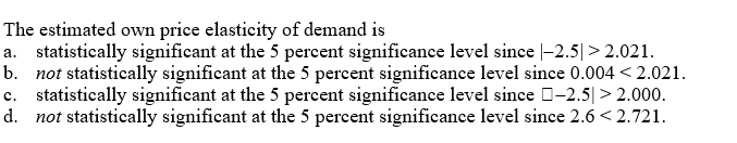
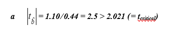
LNP		–1.10	0.44	–2.50	0.0166
LNM		2.40	0.60	4.00	0.0003
LNPR		–0.20	0.05	–4.00	0.0003

These estimates indicate that the demand for the good is

a.      price inelastic since  = -1.10.

b.      price elastic since  = -1.10.

c.      price inelastic since  = -2.5.

d.      price elastic since  = -2.5.

DEPENDENT VARIABLE:	LNQ
OBSERVATIONS:	44
VARIABLE		PARAMETER ESTIMATE	STANDARD ERROR	T-RATIO	P-VALUE
INTERCEPT		–2.00	0.40	–5.00	0.0001
LNP		–1.10	0.44	–2.50	0.0166
LNM		2.40	0.60	4.00	0.0003
LNPR		–0.20	0.05	–4.00	0.0003

DEPENDENT VARIABLE:	LNQ
OBSERVATIONS:	44
VARIABLE		PARAMETER ESTIMATE	STANDARD ERROR	T-RATIO	P-VALUE
INTERCEPT		–2.00	0.40	–5.00	0.0001
LNP		–1.10	0.44	–2.50	0.0166
LNM		2.40	0.60	4.00	0.0003
LNPR		–0.20	0.05	–4.00	0.0003

The estimates indicate that the income elasticity of demand is

a.      -0.20.

b.      -2.0.

c.      2.4.

d.      4.0.

DEPENDENT VARIABLE:	LNQ
OBSERVATIONS:	44
VARIABLE		PARAMETER ESTIMATE	STANDARD ERROR	T-RATIO	P-VALUE
INTERCEPT		–2.00	0.40	–5.00	0.0001
LNP		–1.10	0.44	–2.50	0.0166
LNM		2.40	0.60	4.00	0.0003
LNPR		–0.20	0.05	–4.00	0.0003

The estimates indicate that the income elasticity of demand is

a.      -0.20.

b.      -2.0.

c.      2.4.

d.      4.0.

DEPENDENT VARIABLE:	LNQ
OBSERVATIONS:	44
VARIABLE		PARAMETER ESTIMATE	STANDARD ERROR	T-RATIO	P-VALUE
INTERCEPT		–2.00	0.40	–5.00	0.0001
LNP		–1.10	0.44	–2.50	0.0166
LNM		2.40	0.60	4.00	0.0003
LNPR		–0.20	0.05	–4.00	0.0003

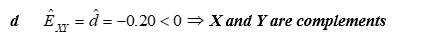
The estimate of the cross-price elasticity indicates that the two goods are

a.      normal goods.

b.      substitute goods.

c.      inferior goods.

d.      complementary goods.

e.      none of the above.

DEPENDENT VARIABLE:	LNQ
OBSERVATIONS:	44
VARIABLE		PARAMETER ESTIMATE	STANDARD ERROR	T-RATIO	P-VALUE
INTERCEPT		–2.00	0.40	–5.00	0.0001
LNP		–1.10	0.44	–2.50	0.0166
LNM		2.40	0.60	4.00	0.0003
LNPR		–0.20	0.05	–4.00	0.0003

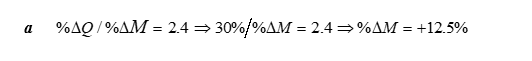
From the above estimates, we would expect quantity demanded to rise by 30 percent if income

a.      rises by 12.5 percent.

b.      rises by 8 percent.

c.      falls by 0.08 percent.

d.      falls by 125 percent.

For a linear demand function, Q = a + bP + cM + dP_R, the income elasticity is

a.   c.

b.   c(M/Q).

c.   c(Q/M).

d.   -c.

e.      -c(Q/P_R).

b - For linear specifications, elasticities vary.  The income elasticity is c(M/Q), where c is constant but M/Q varies.

A representative sample

a.   eliminates the problem of response bias.

b.   reflects the characteristics of the population.

c.   is frequently a random sample.

d.   both b and c.

e.   all of the above.

d     Both are true by the definition of a representative sample.