AP Micro unit 3
1/115
There's no tags or description
Looks like no tags are added yet.
Name | Mastery | Learn | Test | Matching | Spaced | Call with Kai |
|---|
No analytics yet
Send a link to your students to track their progress
116 Terms
production function
the relationship between the available amount of inputs producing a quantity of outputs
short run
[changes over a short term of time] At least one input is fixed
Long run
[changes over a long term of time]
All inputs are variable [can change]
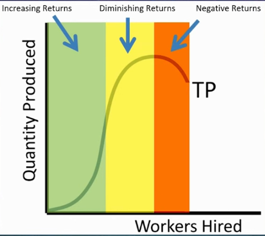
Total Production
amount of output as there are more inputs [workers hired]
![<p>amount of output as there are more inputs [workers hired]</p>](https://knowt-user-attachments.s3.amazonaws.com/b827fc53-1004-42c7-9187-8b947e3929db.jpg)
Total production stages
increasing returns
diminishing returns
Negative returns
Marginal Product
formula
change in TP / QL

Law of Diminishing Marginal returns
“ON which worker does diminishing return set in?”
pick the # of workers it takes to start to see a decrease
Law of Diminishing Marginal returns
“AFTER which worker does diminishing return set in?”
choose the # of workers it takes before the marginal product starts to decrease
Total Product Max
Amount of production reaches its maximum when MP hits the x-axis
Marginal Product
What’s the reason for MP to increase
due to specialization
→ each worker is assigned one specific task to get good at, increasing effective output
Marginal Product
What’s the reason for MP to Diminish
due to more workers spread between a fixed amount of capital
→ multiple people performing the same tasks crowds the effectiveness of the work
Marginal Product
What’s the reason for MP to reach negative returns
More workers get in the way of each other and reduce production
Average Product [AP]
Total production [TP] / Quantity of Labor
MP and AP relationships
when MP> AP = AP is rising
when MP < AP = AP is falling
AP reaches vertex = highest AP
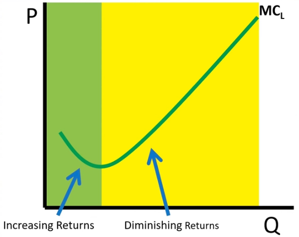
Marginal Cost of Labor [ MCL ]
Wage / MP
→ does not exist at negative return of MP

Marginal Cost of Labor
Graph
Diminishing return sets in at Minimum of function
increasing returns are found when MC decreases
Diminishing returns are found when MC increases
AVG variable cost of labor [AVCL]
# of workers x wage / TP
MCL vs AVC
look at graph

MP and AP vs MCL and AVC
→ When MP rises? When MP falls?
rise = MCL falls
falls = MCL rises
→ are just opposites of each other
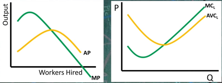
MP and AP vs MCL and AVC
→ When AP rises? when AP falls?
rises = AVC falls
falls = AVC rises
→ are just opposites of each other

Fixed Cost [FC]
price doesnt change w amount of output
fixed cost example
Even if the bakery produces 0 loaves of bread, it still has to pay $2,000 for rent and equipment.
If it produces 1,000 loaves, the rent is still $2,000.
Variable Cost [VC]
price changes with amount of output
variable cost example
Each worker is paid $15 per hour.
If the bakery produces 0 cookies, it hires no workers, so labor cost = $0.
If it produces 1,000 cookies, it might need 5 workers for 8 hours each, costing $600.
→ delete
also known as TFC and TVC
Total cost [TC]
Fixed cost + Variable Cost
TC graph
is the same as TVC but shifted upwards
shifts upward as much as TFC shifts upward

Marginal Cost
change in TC over change in Quantity
VC from MC
VC is the sum of each units MC
Average Variable cost [AVC]
VC/Quantity
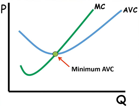
MC and AVC
Graph
AVC will intersect MC at its minimum
AVC drags down when MC drags down
AVC drags up as MC drags up
Average Total Cost [ATC]
TC/Q
ATC and MC
Graph
ATC’s minimum intersects MC
when mc is below ATC → ATC falls
when mc is above ATC→ ATC rises
Productive efficient Q is found at ATC’s minimum [producing at the lowest AVC]
MC = ATC at minimum
![<ol><li><p>ATC’s minimum intersects MC</p></li><li><p>when mc is below ATC → ATC falls</p></li><li><p>when mc is above ATC→ ATC rises</p></li><li><p>Productive efficient Q is found at ATC’s minimum [producing at the lowest AVC]</p></li><li><p>MC = ATC at minimum</p></li></ol><p></p>](https://knowt-user-attachments.s3.amazonaws.com/62a28cd7-1f7b-4bcd-a6e4-4c20fd11caba.jpg)
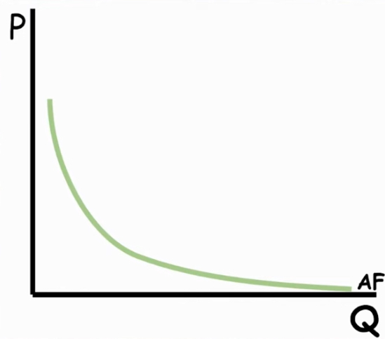
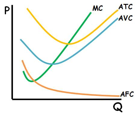
Average fixed cost [AFC]
TFC [total fixed cost]/ Q
AFC
curve on a Graph
FC decreases as Q increases
has an asymptote
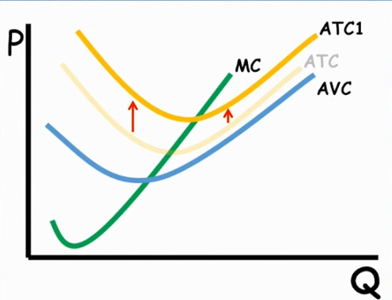
ATC, MC and AVC Graph
A change in the fixed cost
shifts ONLY the ATC upwards
the average fixed cost is the gap between AVC and ATC
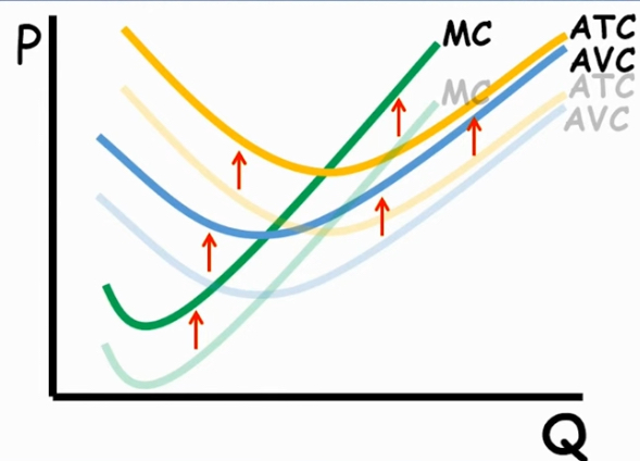
ATC, MC and AVC Graph
Change in Variable cost
all functions shift upwards
ATC, MC and AVC Graph
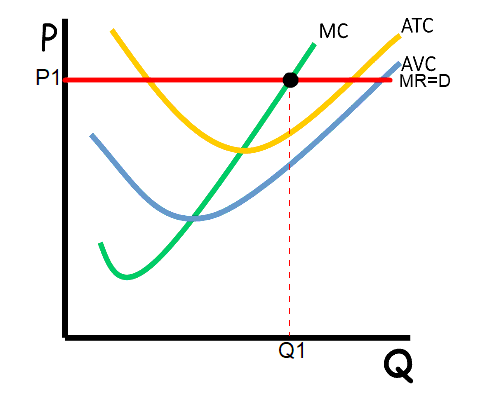
Finding TC via graph
Find production price of either ATC, AVC by finding its y axis point
Multiply it by the quantity [x-axis point]
itll be a rectangle
![<ol><li><p>Find production price of either ATC, AVC by finding its y axis point </p></li><li><p>Multiply it by the quantity [x-axis point]</p></li><li><p>itll be a rectangle</p></li></ol><p></p>](https://knowt-user-attachments.s3.amazonaws.com/28841c14-22ce-4422-96d9-0c924cf552d4.jpg)
ATC, MC and AVC Graph
Finding the cost of production
from the function head down to the quantity and across to the price

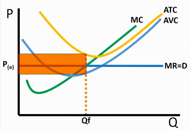
ATC, MC and AVC Graph
finding the average fixed cost
by finding the price of production for ATC and AVC
you subtract the two production costs to find the gap between = AFC
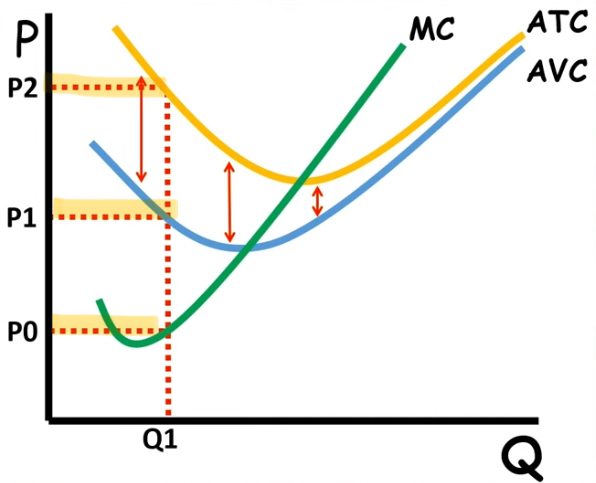
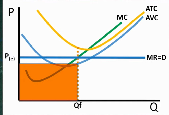
ATC, MC and AVC Graph
finding the TOTAL fixed cost
finding the higher production [p2] multiplying it by Q
then subtract the area of p1 times Q
![<ol><li><p>finding the higher production [p2] multiplying it by Q</p></li><li><p>then subtract<strong> the area </strong>of p1 times Q</p></li></ol><p></p>](https://knowt-user-attachments.s3.amazonaws.com/e43aeec3-d0f4-4ea2-b1d9-06f37cfcd90c.jpg)
Why do ATC and AVC get closer?
bc AFC is always decreasing
why is ATC U-shaped?
as AFC falls it drags down ATC with, but will begin to increase again bc of the rising AVC due to diminishing returns
→ rising AVC outweighs the dragging AFC

When a question is reffering to input/output
its just talking about Quantity itself
AFC, ATC, AVC and MC relation
Graph
what creates Long run ATC
different capacities of production
ATC long run curve
consists of all the minimum short run firms’ ATC’s of different capacities
ATC long run curve
phases
Economies of scale
Constant return of scale
Diseconomies of scale
ATC long run curve
Economies of scale
cost falls as capacity increases
occurs bc of…
Bulk purchase of resources
better capital
better tech
management is efficient
ATC long run curve
Constant Returns to Scale
cost stays the same as capacity increases
operating at an efficient scale
ATC long run curve
minimum efficient scale
is the lowest quantity that minimizes average cost
increasing output has no effect
→ found at constant returns to scale
ATC long run curve
diseconomies of scale
cost rises as capacity increases
occurs when..
communication is having a breakdown
bureaucracy inefficiency [too large for management to continue efficiency]
Returns to scale
If you were to double all inputs, what would occur to the output?
Returns to scale
increasing [economies]
if you double all inputs [labor/capital] =
more than double in output
→found in economies of scale
Returns to scale
constant returns
double all inputs =
exactly double the outputs
→ found in constant returns to scale
Returns to scale
decreasing
double all inputs =
less than double the output
→ found in upwards slope [diseconomies scale]
Minimum efficient scale [MES] vs. market size
mes is small compared to market size
many small firms can operate with perfect competition
Minimum efficient scale [MES] vs. market size
mes is large compared to market
only a few large firms can operate efficiently
Explicit cost
the regular cost of materials or ingredients needed to produce a product
→ fixed + variable cost = explicit
Implicit cost
[Opportunity cost]
The loss of money/time to make other amounts of money → left old job that paid 2k to start a buisiness
Accounting profit
regular profit
total revenue - explicit cost = profit
Economic Profit
total revenue - [implicit + explicit cost] = profit
accounting profit - opportunity cost
Normal profit "breaking even”
economic profit is 0
accounting profit is equal to implicit cost
no entry or exit of market
accounting profit doesnt include
opportunity costs
Why is economic profit important
Accounting profit may look good, but a firm could still be underperforming economically if opportunity costs are high.
Economic profit provides a more accurate picture of whether a firm should continue operating or consider alternative uses of its resources.
In the long run, competitive markets force firms toward normal profit (economic profit = 0).
economic profit >0
positive
Firms
earning more than o.p.c
attracts new firms to enter the market
economic profit < 0
firm consequences
cant cover cost of o.p.c
firm might exit market in the long run
finding marginal product in a table
do not take the output as the amount of MP, rather find the change in output
Profit maximization
TR vs TC
TR > TC = economic profit
TR < TC = economic loss
TR = TR = breaking even [normal profit]
for a firm its not MB
its MR → revenue for producing one product
Marginal revenue
change in TR/ change in Q
when is profit maximization found
MR = MC
MR and MC graph
point of intersection is profit max
MR and MC graph
relations
MR > MC → production increases
MR < MC → production decreases
Profit maximization
when should a firm continue to produce
as long as MR > MC but stop production at MR < MC
MR and MC table FRQ
bc 7$ MR > 6$ MC, but at 5 units 5$ MR < 6$ MC
“revenue from producing one more unit”
referring to MR
MR = MC
graph
the line equals MC = MR = D = P = AR
Notes:-
avc
fixed cost
remember cost and what an item is being sold for are two different things
still has to be paid when facing economic loss
Shut down vs. exit the market
→ temporarily closed in the short run [less hrs ina day]
→ permanently closed
A firm operates when
if not = shutdown
Loss < fixed costs
P=AR > AVC
TR > VC
If a firm shuts down INSTEAD of operating at a loss
what is the loss?
Loss = fixed cost
→ if operating FC + VC
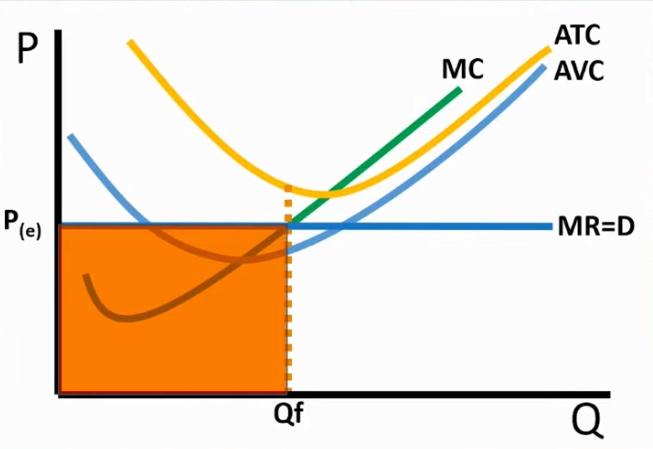
If a firm operates at a total loss
formula
Loss = TR - (VC + FC)
Finding Economic loss
Graph
From the space between ATC and price
Finding the FC
Graph
The rectangle below the price
→ starts from AVC at Qf till price
P > ATC
Short run firm
economic loss is less than fixed cost
→ fixed = red
TVC
Graph
From AVC at Qf and make a square out of it
(Note that it doesn’t line up with price)
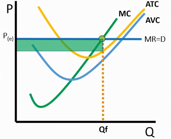
Total rev
Perfect comp firm Graph
Square from price and Q max
If Price over ATC at the profit-maximizing
Earning a profit with no loss for the firm
→ found by (Price - ATC) x Qf
ATC meets MC and P
A firm breaks even
→ if they choose to shut down = loss is found between AVC and ATC till price
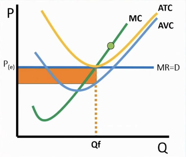
Price is under ATC for a firm but above AVC
Graph
The firm is undergoing economic loss
Economic loss is found between price and ATC
but shutdown is bigger and between ATC and AVC [fixed cost]
economic loss < fixed cost
Price meets AVC in a firm
Shut down point is met
→ shutting down is cheaper than not
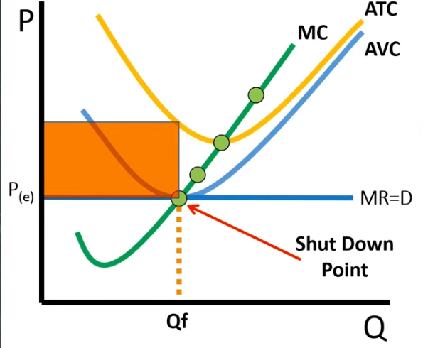
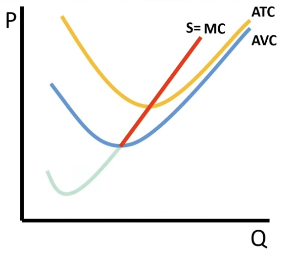
Firms supply curve
MC curve above minimum of the minimum of the AVC curve
How firms get to long run equilibrium
With a starting point of short run profit
→ noting barriers are low
Firm will enter the market → Market supply [not firm] shifts to the right, Price falls → until zero economic profit
How firms get to long run equilibrium
With a starting point of short run loss
→ noting barriers are low
Firms exit the market → Market supply shifts left, Price rises → until zero economic profit
A firm exiting the market as it experiences short run losses in low barrier entry
Permanently shuts down
In the long run
Costs
Are all variable, fixed and variable are all adjustable due to time
Perfect competition
Many buyers and sellers
identical products,
3. a lot of competition,
no barriers to entry
price takers
Perfect competition
long run effect
a firm will always experience zero economic profit
Profit maximization
where price meets MC = MR to determine Qf