11 Lesson 2: Continuous Random Variables, The Continuous Uniform Distribution, The Normal Distribution, and the Lognormal Distribution

How is a Normal Distribution represented?

The normal distribution is defined by its mean (μ) and variance (σ²), written as X ∼ N(μ, σ²).

What are the properties of the Normal Distribution?

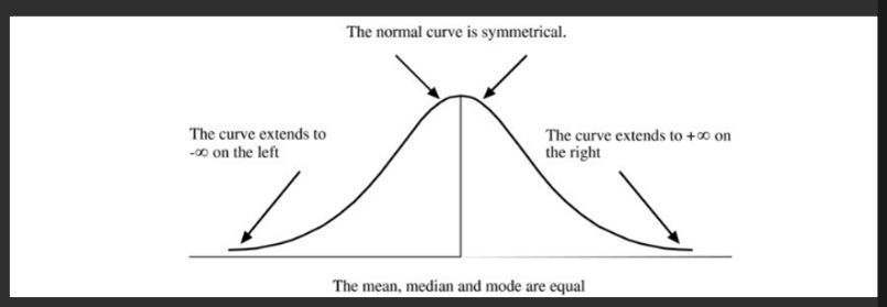
1. Symmetry: It is symmetric around its mean, with a skewness of 0.

2. Equal Tails: The probability that X is less than or equal to the mean is the same as the probability that X is greater than or equal to the mean, both equal to 0.5. The mean, median, and mode are identical.

3. Kurtosis: Kurtosis equals 3, and excess kurtosis equals 0, indicating a specific shape.

4. Linear Combinations: Linear combinations of normally distributed random variables are also normally distributed. For instance, if the returns on individual stocks in a portfolio are normally distributed, the portfolio returns will also be normally distributed.

5. Tail Behavior: The probability of extreme values far from the mean decreases but never reaches zero, with tails extending to infinity.

Graph a Normal Distribution

What is a Univariate Distribution?

Describes the distribution of a single random variable.

What are Multivariate Distribution?

They are linear combinations of normally distributed random variables. This distribution is also normal.

Give and example of a Multivariate Distribution

Portfolio returns with normally distributed individual returns exhibit multivariate normal distribution characteristics.

State the parameters of a Multivariate Normal Distribution (Portfolio)

1. Mean returns for each of the n individual stocks (μ₁, μ₂, ..., μₙ).

2. Variances of returns for each of the n individual stocks (σ²₁, σ²₂, ..., σ²ₙ).

3. Return correlations between each possible pair of stocks, resulting in n(n-1)/2 pairwise correlations. In a portfolio with 4 assets, there are 4 means, 4 variances, and 6 correlations to define the multivariate distribution.

What do Confidence intervals represent?

A confidence interval represents a range of values where a population parameter is expected to exist a certain percentage of the time.

Explain what a 95% confidence interval between 4 and 8 means

There is a 95% confidence that the population parameter falls within this range. Alternatively, there's a 5% chance it doesn't.

What can we say about population parameters?

Population parameters are often unknown, so they are estimated using sample data.

What are the common Confidence Intervals?

1. 90% Confidence Interval: Ranges from ¯x - 1.65s to ¯x + 1.65s.

2. 95% Confidence Interval: Ranges from ¯x - 1.96s to ¯x + 1.96s.

3. 99% Confidence Interval: Ranges from ¯x - 2.58s to ¯x + 2.58s.

Where ¯x is the sample mean and s the sample standard deviation.

Why do we standardize random variables?

Standardization makes it easier to compare different random variables that may have different units or scales. By converting them to a common scale (Standardized variables have a mean of 0 and a standard deviation of 1). This simplifies calculations and statistical analysis.

How is the Z-Score calculated?

z = (observed value - population mean) / standard deviation

What does the Z-Score represent?

Representing how many standard deviations an observation is away from the population mean.

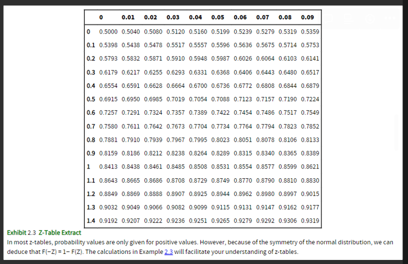
How is the Z-Table used?

Is used to find the probability of and observed value being less than certain standardized value → P(Z ≤ z)

What happens if we want to calculate the complement?

For example, if P(Z ≤ 0.1) is 0.5398

The complement: The probability of returns greater than 0.1 standard deviations above the mean (18%) is 1 - 0.5398 = 0.4602.

State the Z-Table

In most z-tables, probability values are only given for positive values. However, because of the symmetry of the normal distribution, we can deduce that F(−Z) = 1− F(Z).

What is the objective of Roy’s Safety-First Criterion?

The objective of Roy's safety-first criterion is to minimize the probability of the portfolio return (Rp) falling below the target return (RT).

State Roy’s Safety-First Criterion

• RP = Portfolio return.

• RT = Target return.

• P(Rp < RT) = Probability that the portfolio return is less than the target return.

• he z-score or shortfall ratio (SF Ratio) is given by:

  • SF Ratio (z-score) = (E(RP) - RT) / σP

Interpret the Roy’s Safety-First Criterion

SF Ratio represents how many standard deviations the target return is from the expected portfolio return.

What does a higher SF Ratio implies?

A higher SF Ratio implies a better risk-return tradeoff for the portfolio, given the investor's threshold level.

A higher SF Ratio indicates a portfolio with a lower probability of achieving returns below the threshold level.

What is the conclusion of the SF ratio?

Portfolios with *higher* SF Ratios are preferred to those that have a *lower* SF ratio. *Higher* SF Ratio portfolios have a *lower* probability of not meeting their target return

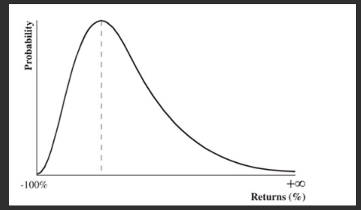
What is a lognormal distribution?

A random variable, Y, follows the lognormal distribution if the natural logarithm of Y, ln(Y), is normally distributed. Conversely, if ln(Y) is normally distributed, then Y follows the lognormal distribution.

Describe the key features of the Lognormal Distribution

1. Lower Bound: The lognormal distribution is bounded by zero on the lower end, meaning that Y cannot take negative values.

2. Upper Bound: The upper end of the distribution is unbounded, allowing Y to take on infinitely large positive values.

3. Positive Skew: The lognormal distribution is positively skewed, indicating that it has a tail on the right side. This means that extreme positive values are more likely than extreme negative values.

Where can we apply Lognormal Distributions?

We can apply this distribution to Holding Period Returns. This because HPR on assets range from -100% (a total loss) to +∞ (unlimited gain).

How is the distribution of the HPR?

The distribution of holding period returns for an asset typically exhibits positive skewness. This means that the likelihood of achieving significantly positive returns is higher than the likelihood of experiencing significantly negative returns.

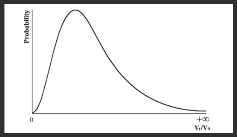
How is the distribution for the the ratio of the ending value of the investment to its beginning value?

The distribution will still be skewed, but with a lower bound of zero, and no upper bound.

0≤Vt/V0≤+∞

Notice that Vt/V0 equals (1 + holding period return)

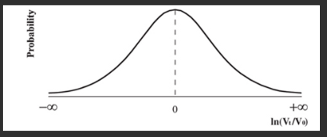
Describe the lognormal distribution of the profitability index (Vt/V0)

The distribution is unbounded at both ends. Bear in mind that ln (Vt/V0) is the same as ln (1 + HPR).

Compare the distribution and the lognormal distribution of (Vt/V0)

While the distribution of the variable (Vt/V0) follows the lognormal distribution, (lower bound = 0; no upper bound), the distribution of the natural logarithm of (Vt/V0) is normally distributed with a lower bound of −∞ and upper bound of +∞.

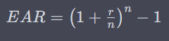
Define the effective annual rate (EAR)

Is a way to express the annual interest rate on financial products that compound interest more frequently than once per year. It reflects the true annual interest rate, including the effect of compounding.

Describe the relationship between compounding periods (n) and EAR

As the compounding periods get shorter and shorter, the effective annual rate (EAR) rises

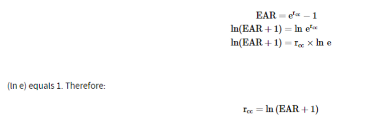
State the EAR formula with a continuous compounding

Calculate the EAR with a stated rate of 5% using the TI BA II calculator

The TI BA II keystrokes for solving (e0.05 − 1) are: “0.05” \[2nd\] \[ln\] \[-\] “1”

Find and expression of the continuously compounded annual rate in function of EAR

What relationship exists between continuously compounded returns and lognormal asset prices?

If continuously compounded returns are normally distributed, asset prices are lognormally distributed

Why is the central limit theorem important in finance when considering asset prices?

It implies that continuously compounded returns don't need to be normally distributed for asset prices to be reasonably well described by a lognormal distribution.

State the relationship between rcc with HPR and Vt/V0

rcc=ln(1+HPR)

(1 + HPR) simply equals (Vt/V0). Therefore, the continuously compounded rate of return can also be calculated as:

rcc=ln(Vt/V0)

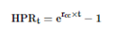
State the relationship between HPR and the continuously compounded rate

State the key properties of the Student’s t-Distribution

1. Symmetry: The t-distribution is symmetrical around its mean, just like the normal distribution.

2. Degrees of Freedom (df): It is defined by a single parameter, the degrees of freedom (df), which is equal to the sample size minus one (n - 1). The degrees of freedom determine the shape of the t-distribution.

3. Shape: The t-distribution has a lower peak than the normal distribution, which means it has fatter tails. As the degrees of freedom increase, the t-distribution approaches the shape of the standard normal curve.

4. Effect of Degrees of Freedom: As the degrees of freedom increase, the t-distribution curve becomes more peaked and its tails become thinner, resembling the normal curve more closely.

What is the relationship between the degrees of freedom and confidence intervals on a t-student Distribution?

As the degrees of freedom increase, the t-distribution approaches a normal distribution. Consequently, for a given significance level, the confidence interval for a random variable following the t-distribution becomes narrower when the degrees of freedom increase. This indicates increased confidence that the population mean lies within the calculated interval.

When can we use the t-distribution?

• It is used to construct confidence intervals for a normally (or approximately normally) distributed population whose variance is unknown when the sample size is small (n ﹤ 30).

• It may also be used for a non-normally distributed population whose variance is unknown if the sample size is large (n ≥ 30). In this case, the central limit theorem is used to assume that the sampling distribution of the sample mean is approximately normal.

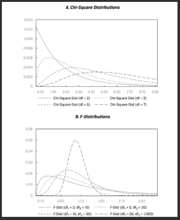
State the key properties of the Chi-Square Distribution

1. Asymmetrical Distribution: The chi-square distribution is asymmetrical in shape.

2. Degrees of Freedom: The chi-square distribution with k degrees of freedom is defined as the distribution of the sum of the squares of k independent standard normally distributed random variables. It is a family of distributions, with a different distribution for each possible value of degrees of freedom.

3. Non-Negative Values: The chi-square distribution does not take on negative values, as it involves the sum of squared values.

State the key properties of the F-Distribution

1. Family of Distributions: Similar to the chi-square distribution, the F-distribution is a family of probability distributions.

2. Numerator and Denominator Degrees of Freedom: Each F-distribution is defined by two values of degrees of freedom: the numerator degrees of freedom (df1) and the denominator degrees of freedom (df2).

3. Relationship to Chi-Square: The F-distribution is related to the chi-square distribution. If χ²₁ is a chi-square random variable with m degrees of freedom, and χ²₂ is another chi-square random variable with n degrees of freedom, then F = (χ²₁/m) / (χ²₂/n) follows an F-distribution with m numerator and n denominator degrees of freedom.

4. Bell Curve Shape: Similar to the chi-square distribution, as the degrees of freedom increase for the F-distribution, its probability density function becomes more bell curve-like.

Graph the Chi-Square and F-Distributions