Econ 101 (final)

microeconomics

Explicit Cost

cost that involves monetary payments to acquire goods or services; we actually paid this cost

ex. paying $2 for a coffee

Implicit Cost

cost that doesn’t involve monetary payments; ‘opportunity cost’

ex. losing 15 by waiting in a drive-thru “lost earning, which could have been earned if you worked the 15 minutes”

Total cost in accounting

explict cost (‘reciepts’), no implict cost

ex. $2

Total cost in economics

explicit cost + implict cost

ex. $2 (explict) + $10 (implicit) = $12

Comparison of economics/accounting cost/profit

Sunk/’dead’ cost

cost that once incurred (happens), it cannot be recovered

ex. paint on a car (can’t restore it)

• since you cannot recover this cost, they become irrelevant and we should ignore it in making future decisions (don’t let it affect your decisions)

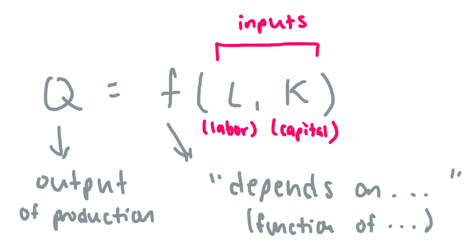
Production

how much ‘output of production’ we could have depends on how much inputs are available

• for simplicity, we will assume we only have 2 inputs (labour (L), and capital (K))

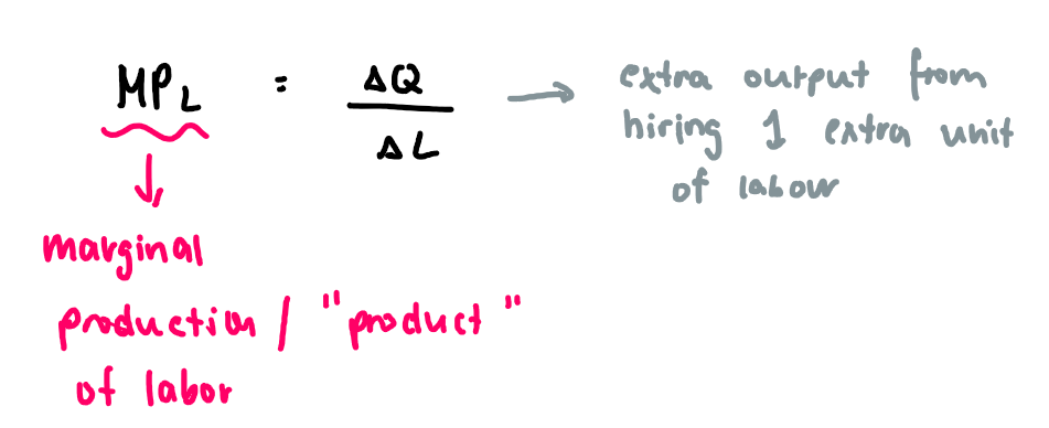
Marginal production formula (on formula sheet)

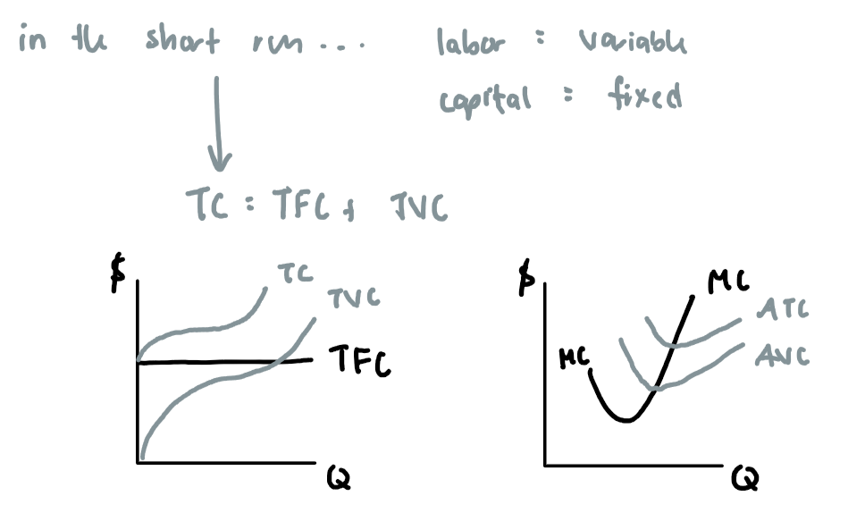
Production/inputs in the short run

capital is fixed (b/c changing capital takes time, not easily changed), but labour is variable

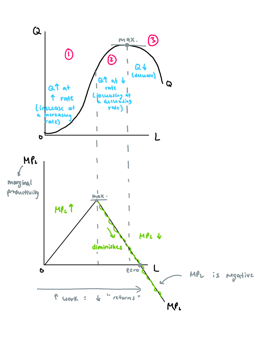
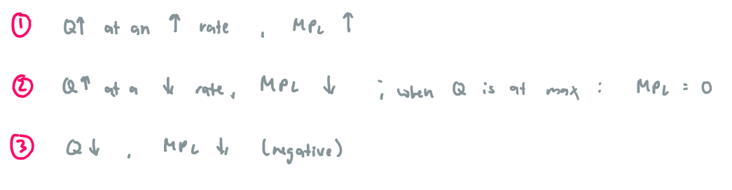
Short run production has three stages

First stage: increasing returns, second stage: diminishing returns, third stage: negative returns.

Law of diminishing/decreasing marginal productivity/returns

MP of the variable input/’labour’ will eventually diminish/’decrease’ as we hire more of that variable (labour) input beside a fixed amount of the otther input (capital)

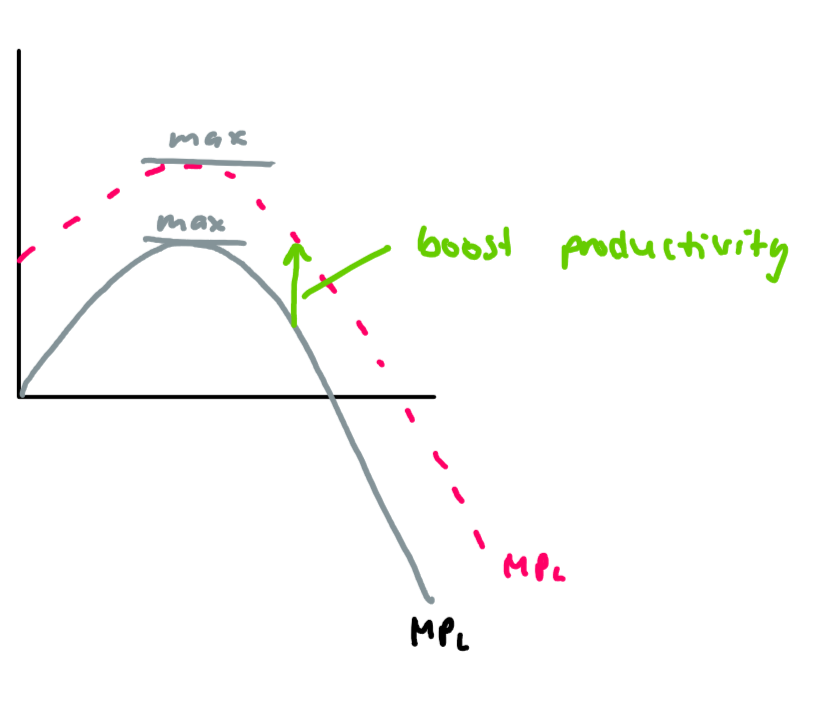
What causes MP_L to ‘shift up’/increase

1. capital “K” increases ex. bigger land

2. technology increases

(the opposite would cause a decrease)

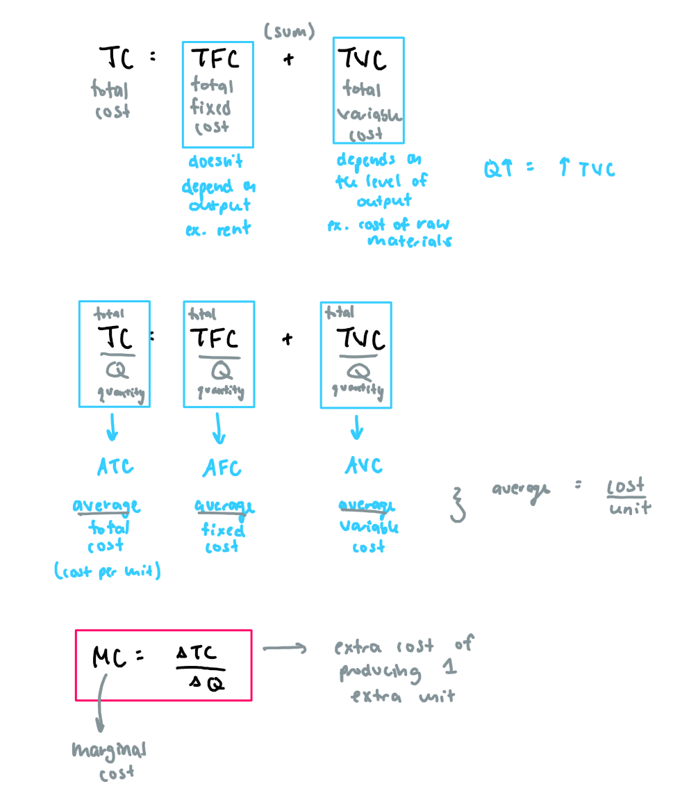
Costs in the short run

refers to all costs that vary with production output, including fixed and variable costs

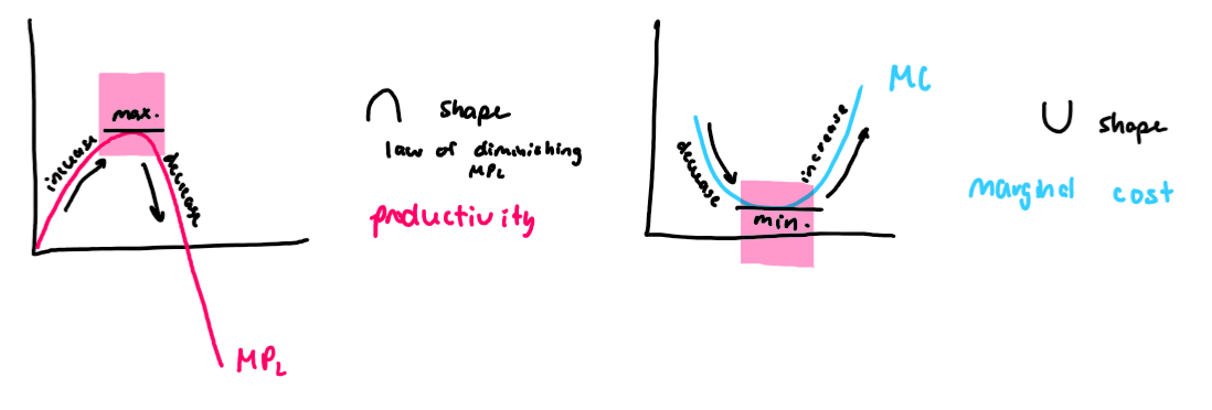
Why is the cost (MC) curve a ‘u shape?

because it is a reflection of the productivity (MP) curve (n shape)

law of diminishing returns is responsible for the shapes of these curves

T or F; when AVC is falling, MC is also falling

false; when AVC is falling MC is rising for part of it

T or F; when MC is falling, AVC is also falling

true

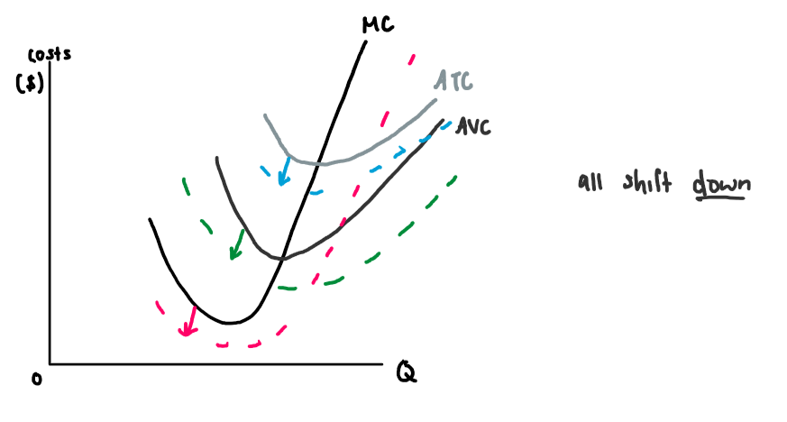
Shifts in the short-run cost curves

if..

1. P_inputs decrease ex. raw materials

2. Taxes (on producers) decreases

3. Less regulations (b/c regualtions increase cost of production)

4. Technology increases (production is more efficient)

all of these will cause the cost of production to decrease, supply increases

MC, AVC, ATC all decrease (all shift down)

and vice versa

• the opposite is also true

  • P_input increases

  • Taxes increases

  • more regulations

  • technology decreases

  all of these cause the cost of production to increase, supply decreases

  MC, AVC, ATC all increase (all shift up)

Production/inputs in the long run

all inputs (labour and capital) are variable (since you have plenty of time to change capital)

Costs in the long run

• no longer have anything fixed

• in the long run, all inputs (L and K) are variable (capital is now variable as well (lots of time to change it)). In this cause, the producer will use the combination of inputs that produces what it wants with the lowest cost

  • the firms will be producing with the lowest cost b/c capital can be adjusted!

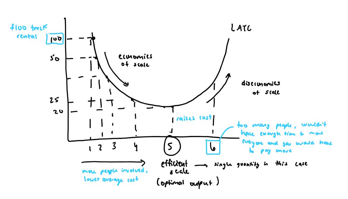
Example of LATC

Long-run in comparison to short-run

In economics, the long-run refers to a period in which all factors of production and costs are variable, allowing firms to adjust all inputs. In contrast, the short-run is characterized by at least one fixed input, limiting the firm's ability to change production levels.

LATC (long-run average total cost)

shows the lowest cost of producing ouput level; it is the lower envelope/carrier of all shortrun total cost curves

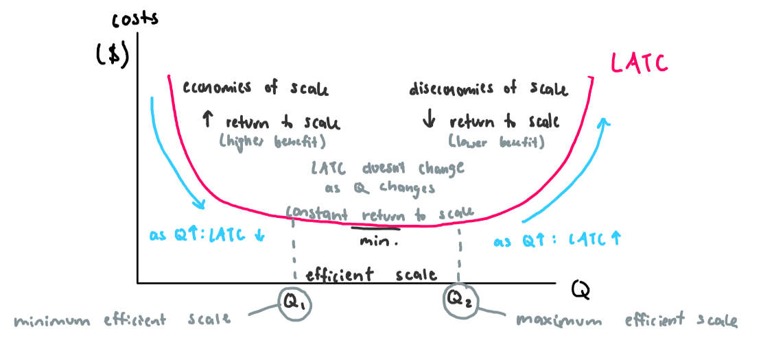
(‘enjoying’) Economies of scale

increased return to scale; as Q increases “scale/size of production” = LATC decreases; bigger scale = decreased cost (cost of savings from bigger scale of production)

Diseconomies of scale

decreased return to scale; as Q increases “scale/size of production” = LATC increases; bigger scale = increased cost (no cost of savings from bigger scale of production)

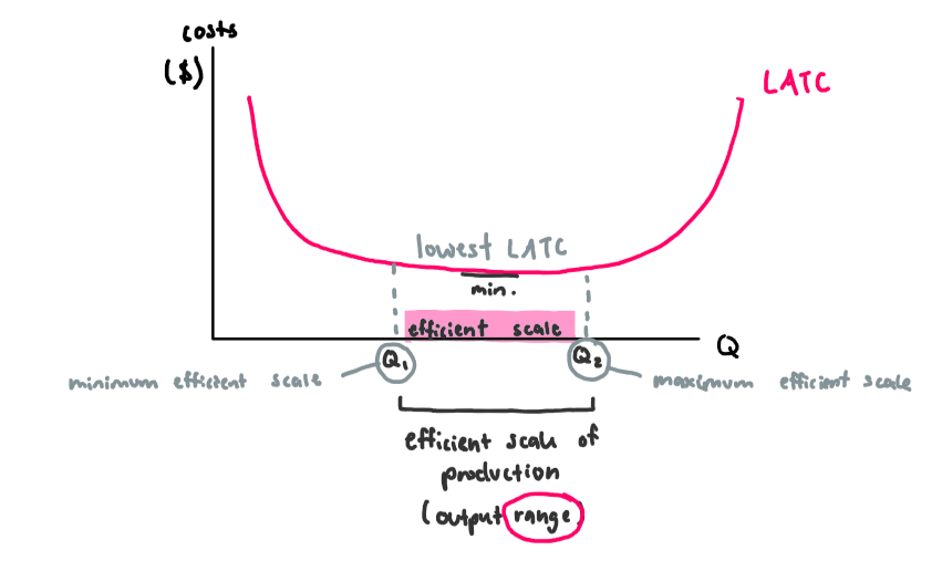
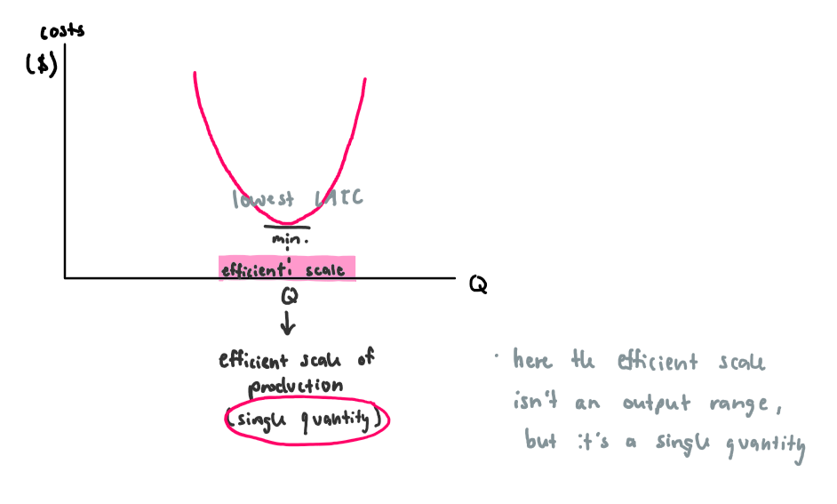
Efficient Scale

constant return to scale; it is the output range at which LATC is at/reaches its minimum

2 types of efficient scales

1. range

spans at the lowest LATC; minimum efficient scale and optimal/maximum efficient scale

2 types of efficient scale

2. single point

is a single quantity at the lowest LATC

Different market structures

1. perfect competition

2. monoply

3. monopolistic competetion

Characteristics of Perfect Competetition

1. large number of sellers and buyers (very many firms)

2. sellers sell identical ‘homogenous’ products

3. no single seller controls the price - it is the whole market (D and S) that determines the price and once the market determines the price, each seller has to accept/take it. Sellers are price takers

   • zero monopoly power

4. free entry and exit; ‘no barriers to entry’

   • any producer can enter the market or exit/’leave’ freely and no one can prevent him

   • monopolists try to protect their monopoly by putting barriers

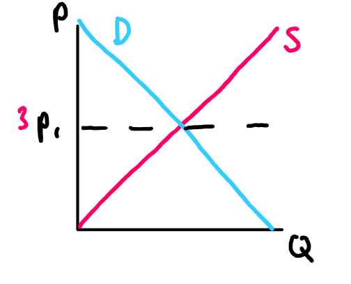
Market

determines the price; price maker

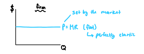
Firm

is a price taker

• firm is forced to charge/sell at the market price (price taker)

• can sell what you want but can’t charge more than what is set

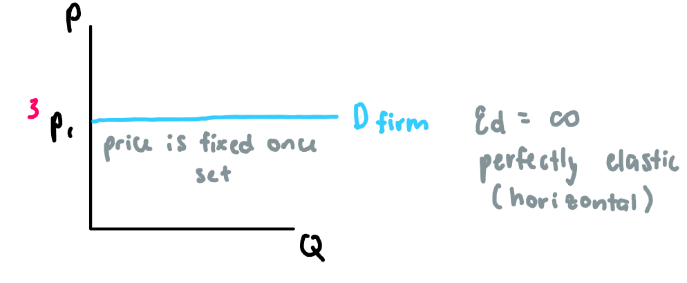
Demand curve

• for a market ‘industry’ = negatively sloped

• for a firm = perfectly elastic (horizontal)

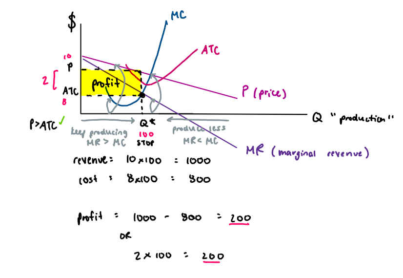
Profit formula

= total revenue (TR) - total cost (TC; economic cost= implict cost + explict cost)

Scenarios

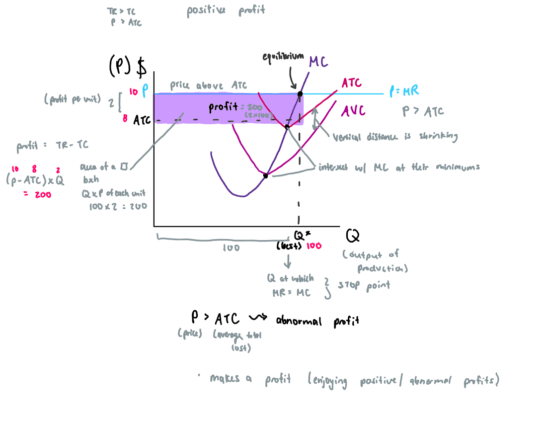
1. profit

   • TR > TC

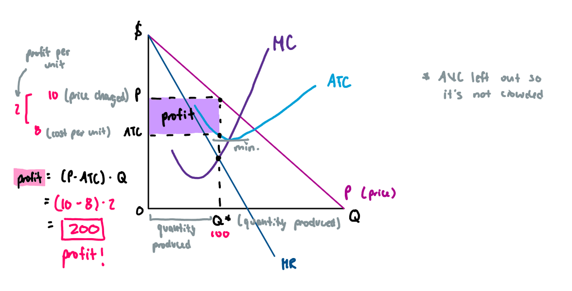
   • P (revenue per unit) > ATC (cost per unit)

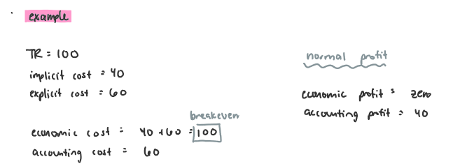
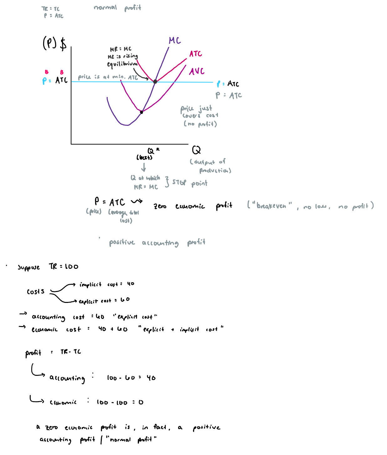
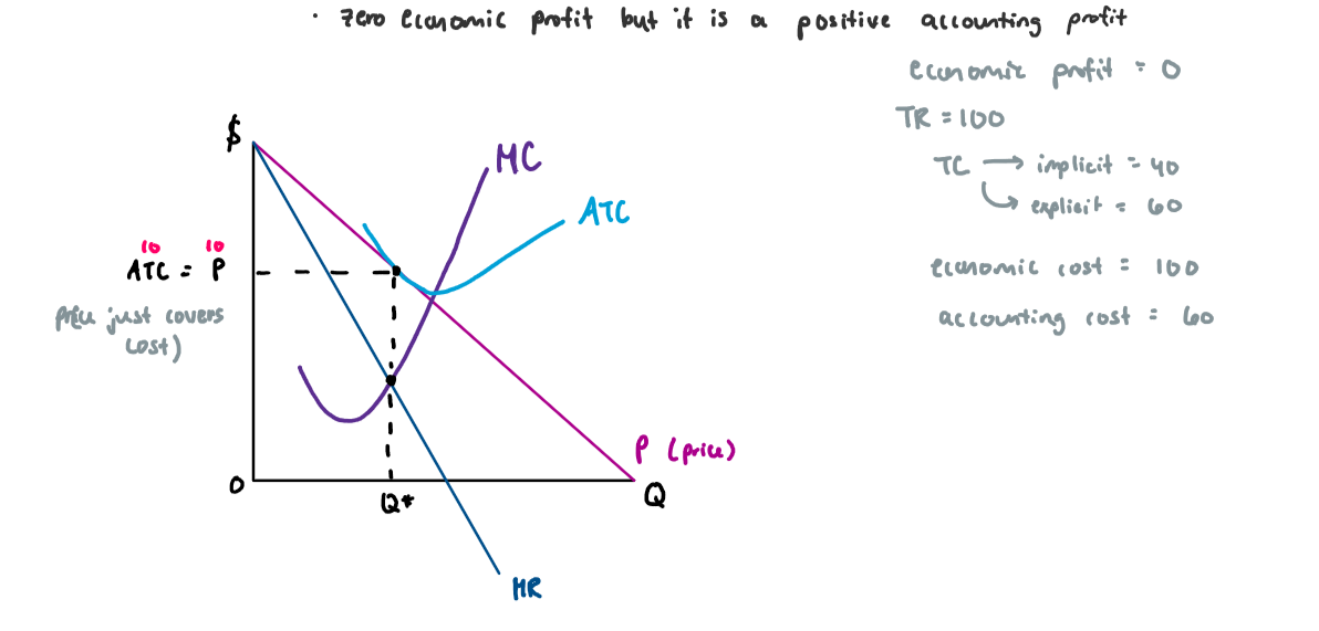
2. breakeven

   • ‘normal profit’

   • TR = TC

   • P = ATC

   • economic profit = 0

   • accounting profit = +

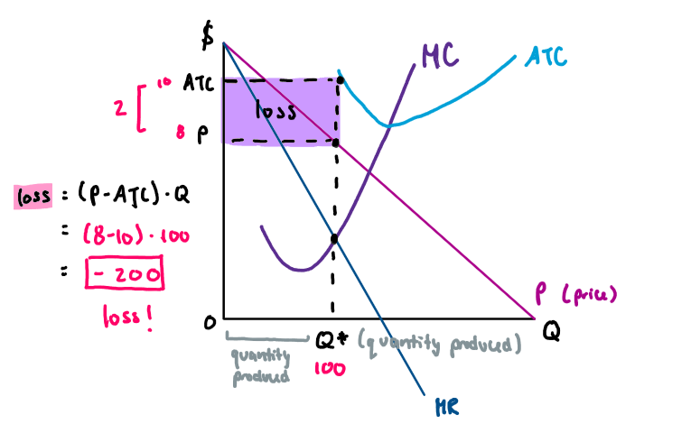
3. loss

   • TR < TC

   • P < ATC

Objective of any producer…

maximize his profits

• trying to produce the best quantity that maximizes your profits or, if you’re suffering from a loss, the quantity will minimize your loss

• profit = TR - TV

Objective of any consumer…

maximize utility/satisfaction

Profit maximization using MR and MC (2 conditions must be satisified)

1. MR = MC (necessary condition)

2. MC is rising (sufficial condition)

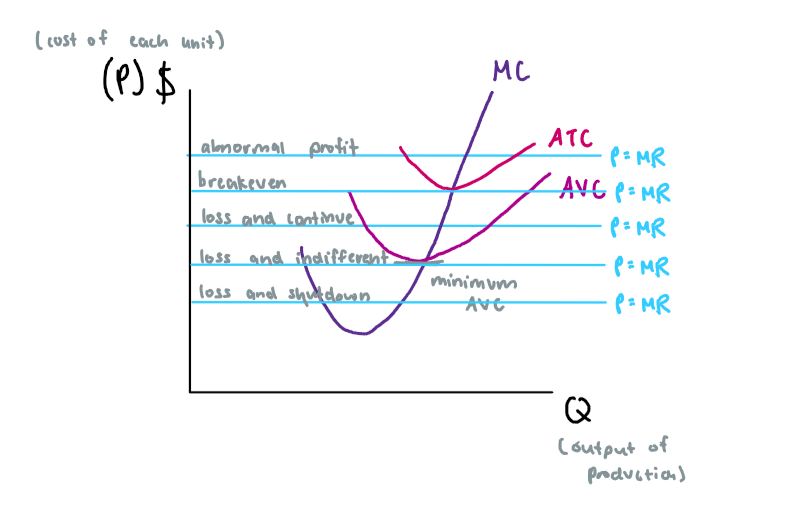
Short-run Equilibrium of a perfectly competitive firm… case 1: abnormal profit

occurs when price is greater than average total cost, leading to maximum profit in the short run

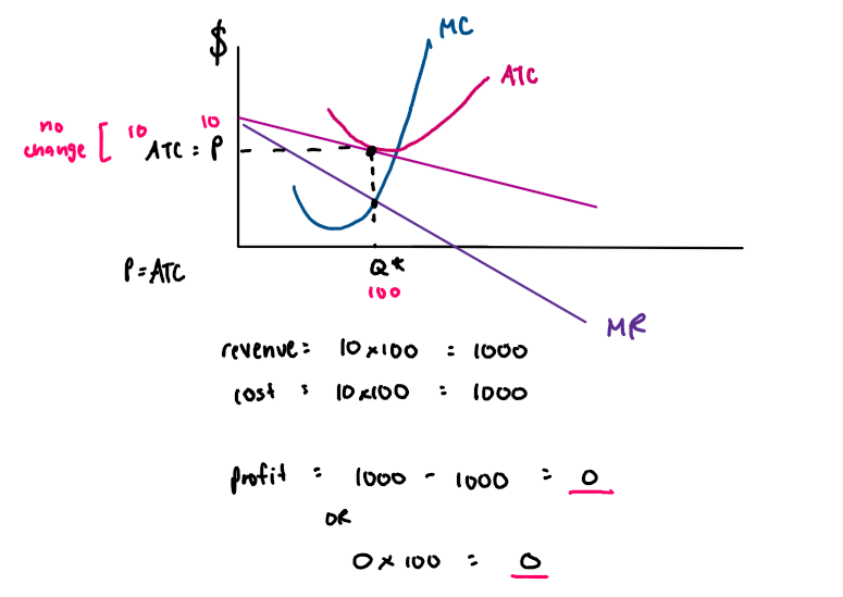
Short-run Equilibrium of a perfectly competitive firm… case 2: breakeven aka normal profit

occurs when price equals average total cost, resulting in no economic profit or loss

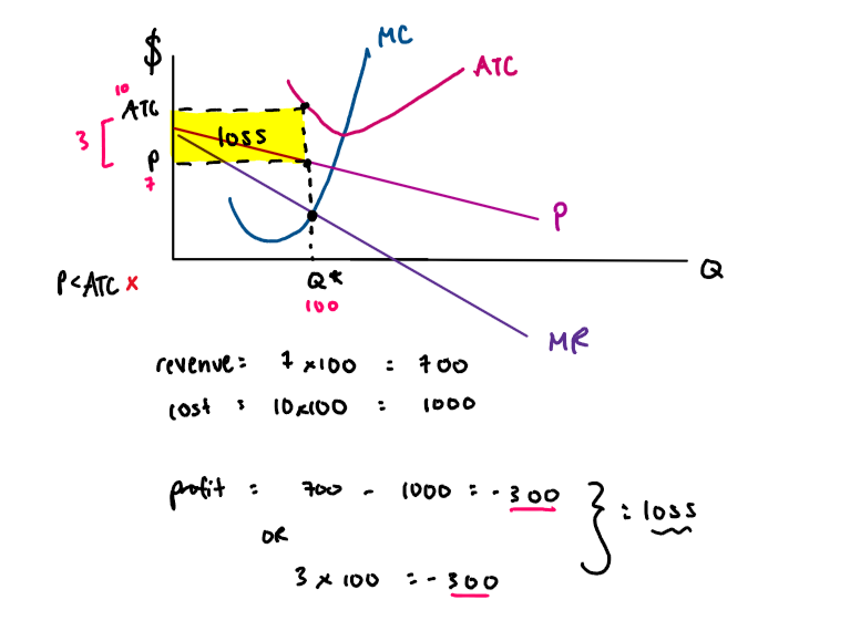
Short-run Equilibrium of a perfectly competitive firm… loss: 3 cases

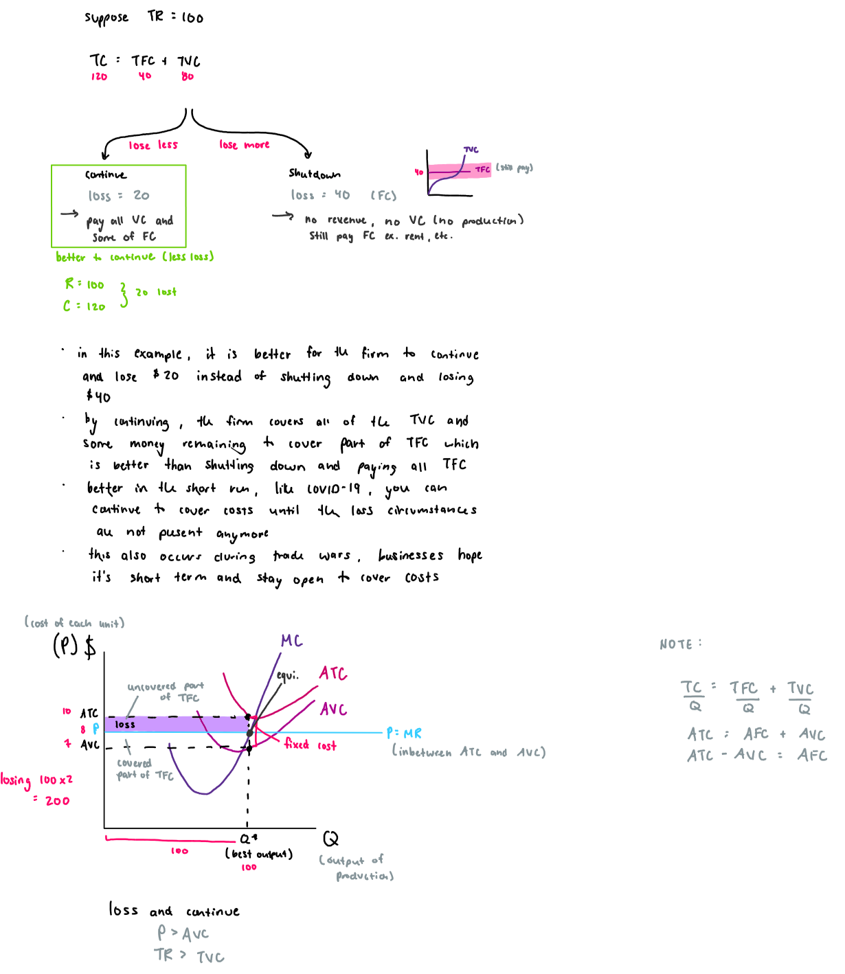
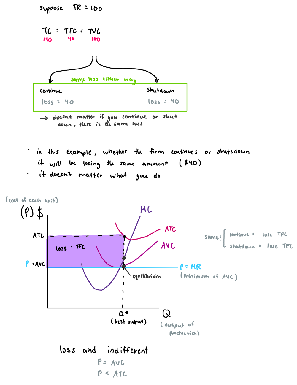
1. loss and continue: TR > TVC, P > AVC “covers costs”

2. loss and indifferent: TR = TVC, P = AVC “just covers costs”

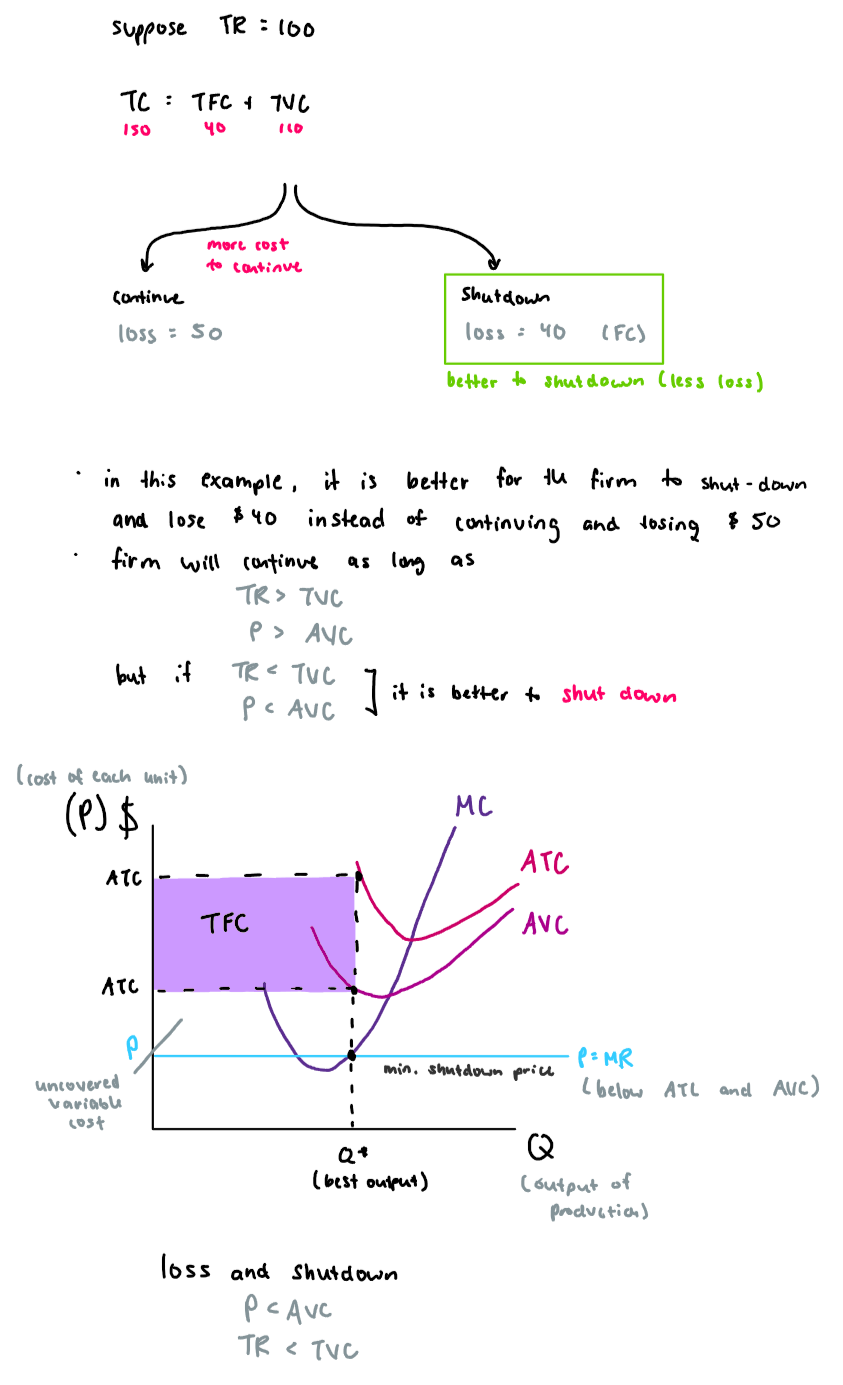
3. loss and shutdow: TR < TVC, P < AVC “didn’t cover costs”

Short-run Equilibrium of a perfectly competitive firm… loss: case 1: loss and continue

*short run only!

The firm continues to operate even though it is incurring a loss, as total revenue covers variable costs and contributes to fixed costs.

Short-run Equilibrium of a perfectly competitive firm… loss: case 2: loss and indifferent

*short run only!

The firm operates at a loss without incentive to exit the market, as total revenue just covers variable costs.

Short-run Equilibrium of a perfectly competitive firm… loss: case 3: loss and shutdown

*short run only!

The firm decides to exit the market as total revenue does not cover variable costs, resulting in losses.

Summary of all cases

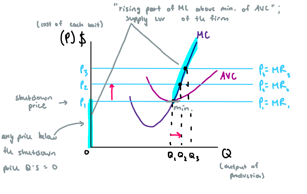
Shutdown price

is the minimum of the average variable price (AVC); if the price goes below it, the firm will shut down indicating it cannot cover variable costs

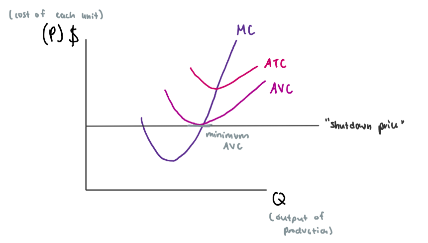
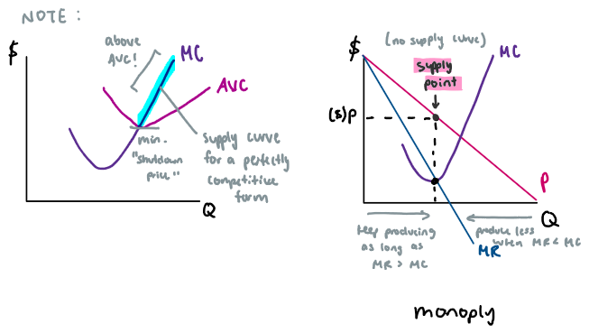
Short-run supply curve of a perfectly competitive firm

the supply curve of a perfectly competitive firm is the rising part of the MC curve above the minimum AVC

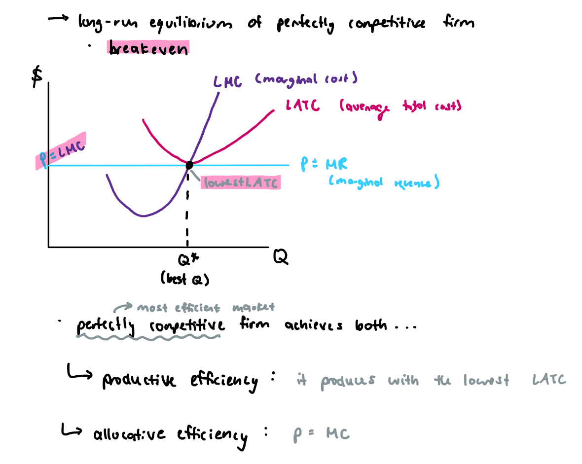
Long-run Equilibrium of a perfectly competitive firm

in the long-run, the perfectly competitive firm will be ‘breaking even’ (normal profit) because of the free entry and exit

• suppose there is a profit, the market is effective and new firms enter the market. They contine to enter as long as there is a profit in the industry (attractive). They continue to enter, more seller, so supply increases and price decreases until profit disappears.

• if there is a loss, firms start to leave until the loss disappears

• in long-run equilibrium, a perfectly competitive firm will achieve both productive (produce with the lowest ATC) and allocative (P=MC) efficiency

A perfectly competitive firm could have…

1. long-run (1 case)

   • breakeven (due to free entry and exit)

2. short-run (5 cases)

   • abnormal profit

   • breakeven

   • loss

     • loss and continue

     • loss and indifferent

     • loss and shutdown

Is a perfect competition economically efficient?

yes! it is the most efficient market style

We have two types of efficiency…

1. productive efficiency

2. allocative efficiency

Productive Efficiency

to produce with the lowest ATC

Utilize resources optimally

Allocative Efficiency

P = MC

This occurs when resources are distributed in a way that maximizes total welfare, ensuring that the price consumers are willing to pay equals the marginal cost of production.

“Free” competitive market

no intervention from the government

where prices are determined solely by supply and demand, leading to optimal resource allocation.

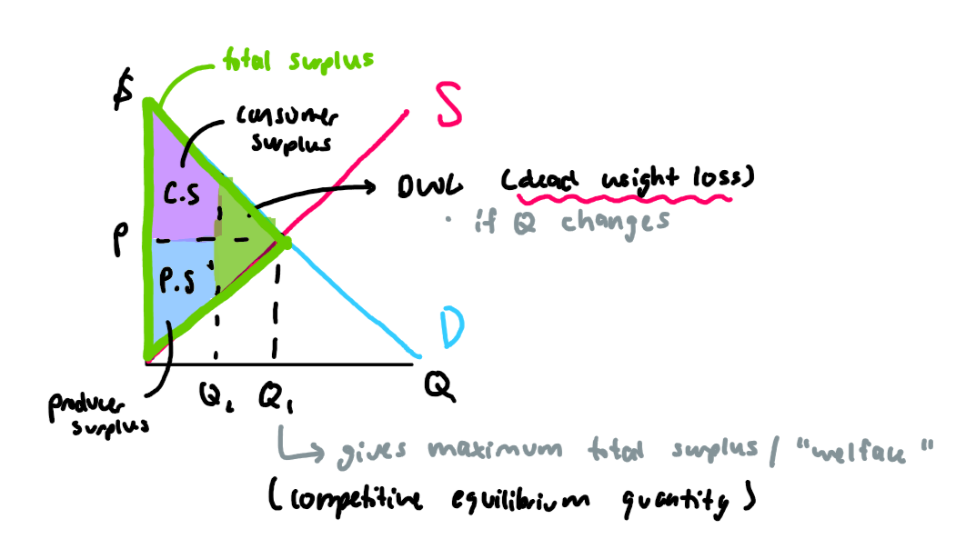
Competitive quantity

maximizes total surplus/welfare

• but at any other quantity other than the competitive equilibrium quantity, it willgive us less total surplus, there will be DWL (dead weight loss)

Market Structures

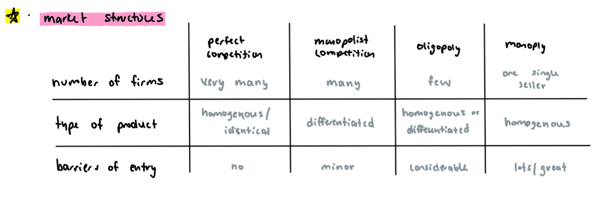
Characteristics of Monopoly

• monopolies are bad!

  1. 1 single seller “price maker” (faces the whole market demand)

  2. product has no close substitutes (homogenous)

  3. great barriers to entry

     • legal- copyright, patent, etc.

     • technical (you are the only one who knows the secret of doing the job)

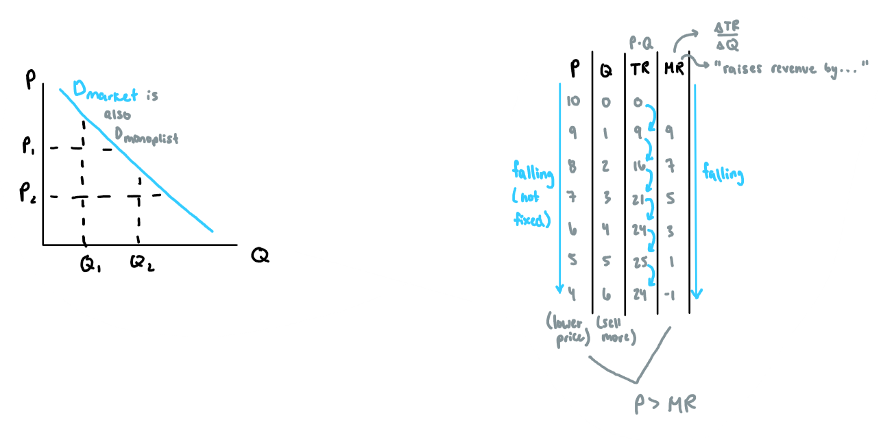
  4. since the monopolist is the only seller in the market the demand for his good is the demand of the whole market

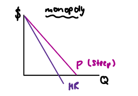
Demand of Monopoly

negatively sloped

to sell more, the monopolist must lower the price to encourage sales

Total revenue (TR) is maximized when…

MR = 0 (no more extra revenue)

Profit is maximized when…

MR = MC

and MC is rising

Supply ‘curve’ of a monopolist vs perfect competition…

monopolist does not have a supply curve, like perfect competition; he has a supply point because the monopolist sets the price based on demand

• the supply point is the point on his demand curve above the intersection of MR and MC

Monopoly… case 1: abnormal profit

occurs when a monopolist sets prices above marginal cost, leading to higher profits than in competitive markets

Monopoly… case 2: breakeven “normal profit”

occurs when a monopolist sets prices equal to marginal cost, resulting in no economic profit but covering all costs

Monopoly… case 3: loss

occurs when a monopolist sets prices below average total cost, leading to economic losses despite generating some revenue

Monopoly power

the ability to charge a price higher than MC

= P - MC (measures the ability of a firm to charge a price higher than MC)

• perfect competition has no monopoly power, P = MC

Monopoly is bad because…

• a monopolist produces a smaller Q and charges a higher price compared to perfect competition

• P ≠ MC, monpolist doesn’t achieve allocative efficiency

• monopolist doesn’t produce with the lowest ATC, monopolist doesn’t achieve productive efficiency

• monopolist creates welfare loss (DWL)

Since monopoly is so bad, how do we prevent it?

1. Anti-combine'/’trust’ laws

2. Government regulations

   • marginal cost pricing

   • average cost pricing

Anti-combine'/’trust’ laws

laws that prohibit monopoly practices by imposing fines or applying criminal laws on monopolies

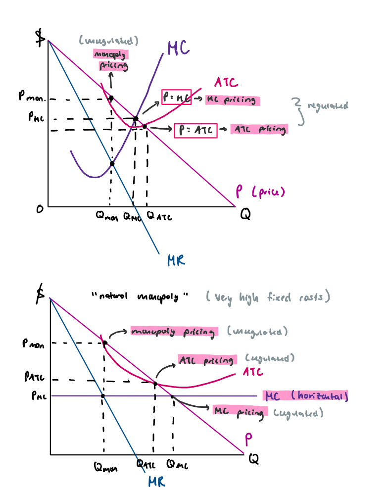
Government regulations

monopolist is not free to charge the price that he wants; the government forces monopolist to charge a specific price

Marginal cost pricing

government forces the monopolist to set P = MC

Average cost pricing

government forces the monopolist to set P = ATC

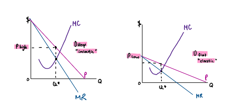
Price discrimination/’differentiation’

• charging different prices for the same good

• charge high price for people who have D_inelastic (don’t care as much, not sensitive, ‘exploit’ consumers)

• charge low price for people who have D_elastic (get upset quickly, sensitive)

Conditions for price discrimination

1. there must be a monopoly power (doesn’t work for perfect competition)

2. market segregation: charge different prices based on difference in elasticities

   • people with elastic demand = low price

   • people with inelastic demand = high price

3. resale is not possible

   • it not be possible to get the good from the cheaper market and resell it in the expensive market to make money/profit off of it

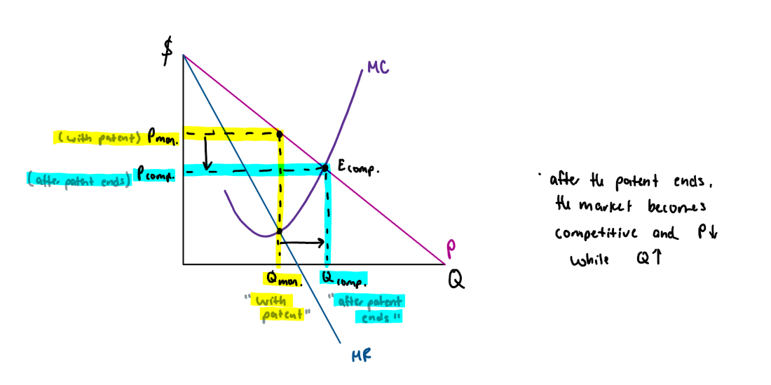
Patent (‘copyright’)

• you are protected for some time

• you behave as a monopolist for some time (you are the only one who can produce an item)

impact of a patent

• the patent protects the producer from competition for a certain period of time. In Canada, it is 20 years. During this period, you will act as a monopolist. But after the patent period ends, the market will be perfectly competitive

Characteristics of Monopolistic Competetition

1. large number of buyers and sellers

2. free entry and exit (causes breakeven in the long-run)

3. products are differentiated (are different/not identical)

4. each firm sets its own price, a firm has some, limited monopoly power

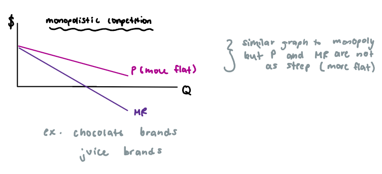
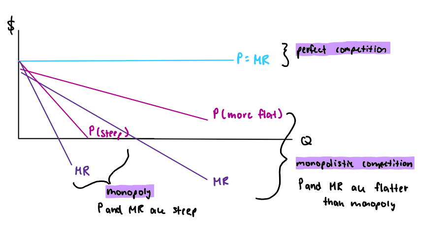
Comparison of perfect comp., monopoly, and monopolistic comp.

perfect comp.: P=MR

monopoly: P and MR are steep

monopolistic comp.: P and MR are flatter than monopoly

Supply ‘curve’ of a monopolist competitive firm…

has no supply curve, similar to monopoly, but has a supply point

Short-run Equilibrium of a monopolistic competitive firm… case 1: abnormal profit

occurs when price exceeds average total cost, leading to positive economic profits for firms in the short run

Short-run Equilibrium of a monopolistic competitive firm… case 2: breakeven (“normal profit”)

occurs when price equals average total cost, resulting in zero economic profits for firms in the short run

Short-run Equilibrium of a monopolistic competitive firm… case 3: loss

occurs when price is below average total cost, resulting in negative economic profits for firms in the short run

Long-run Equilibrium of a monopolistic competitive firm

• due to the free entry and exit: in the long-run, all monopolistic competitive firms will acheive breakeven (‘normal profit’) - no loss and no profit

• if there are profits: new firms will enter the market, these new firms will take some of your customers, D and MR decreases on my product, this entry keeps going until profits disappear

• if there are losses: some existing firms will exit/’leave’, their customers switch to remaining firms, D and MR increase on remaining firms, this exit keeps going until the loss disappears

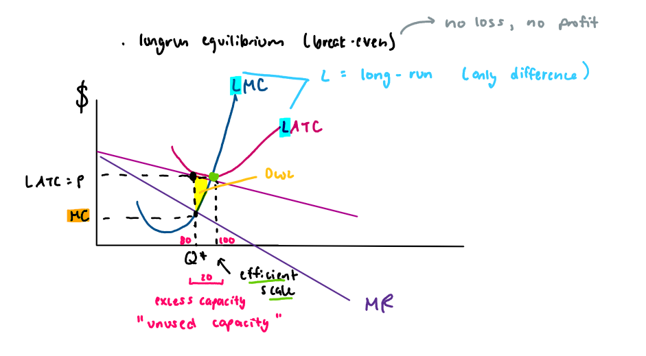
Does monopolistic competition achieve efficiency?

1. productive efficiency: NO; b/c it does not produce with the lowest LATC

2. allocative efficiency: NO; b/c P ≠ MC

note: the only market structure that achieves both allocative and productive efficiency is PERFECT COMPETITION

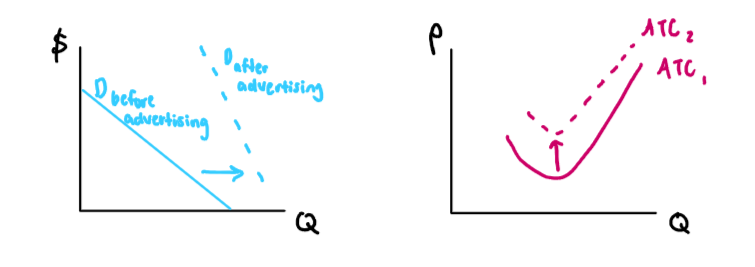
Effect of advertising

• each firm tries to advertise to get more customers

• advertising causes…

  1. increased demand and MR, become steep “inelastic”; customers will be more attracted to you if you advertise

  2. increased ATC; “shift up”; advertising costs money to the firm

Characteristics of an Oligopoly

• few sellers that compete

• sell similar or differentiated products

• high barriers to entry (high costs, small market)

• mutual interdependence

  • when a firm decides its policy, it takes into account the reaction of other firms (competitors)

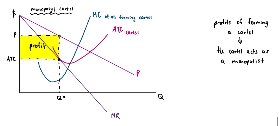
Cartel

is a group of firms that act together by coordinating their decisions

• if all firms formed a cartel, they will act as a monopolist and this gives them higher profits than competing

Why is ‘forming a cartel’/colluding not possible?

1. it’s illegal due to antitrust laws (antimonopoly laws) - illegal to form a monopoly

2. each firm will have an incentive to cheat or deviate as long as there is no binding contract

Payoff matrix

table (given in Q); is a tool used in game theory to show the possible outcomes of a strategic interaction between firms, highlighting the potential profits or losses associated with different actions taken by those firms.

A game consists of…

1. players

2. strategies (‘options’)

3. payoff (‘outcomes for every combination of strategies’/combinations, outcomes, returns)

The first number in each cell belongs to the player on the…

LEFT

The second number is the payoff to player on the…

TOP

Pareto optimal/’efficient’ outcome

cooperative outcome of the game; is the outcome that makes both or at least one of the players better off without making someone else worse off

• although it’s a better outcome for both, both firms won’t go for it (it’s not stable, people deviate/cheat)

Nash equilibrium

noncooperative outcome; is the outcome of the game where none of the players have an incentive to deviate/move away from it

Dominant strategies

are strategies that yield a higher payoff for a player regardless of what the other players choose (better strategy no matter what). In games with dominant strategies, a player will always opt for their dominant strategy to maximize their outcome.