Microeconomics ECON0013

homotheticity (definition?)

Under the Marshallian, how do we determine homotheticity if given…

1. ICs?

2. Utility fxn?

3. MRS?

4. Demand?

constant MRS along rays from origin

1. if within indifference curve function: q1 and q2 have a common scaling

2. Utility fxn is homogeneous u(kx) = ku(x)

3. MRS is only a fxn of ratio x1 and x2. NO tack-ons

4. homogenous to income only, i.e. the fxn is y times some function of p’

quasilinearity, definition?
Identification for Marshallian under

1. ICs

2. Utility fxn

3. MRS

4. Demand

(QUASILINEARITY WRT Q1)

constant MRS along y=c or x=c

1. ICs: find the slope (MRS)

2. Utility fxn has q1 “tacked on”

3. MRS only depends on q2

4. Demand FOR Q2 depends only on p’ without regard to y

quasilinearity (identification from marshallian demand)

if quasilinear wrt good 1, then the Marshallian demand for GOOD 2 will depend on some function of p1 and p2 alone, WITHOUT regard to income

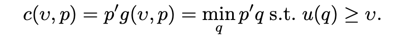
hicksian demand

aka. compensated demand

q* = g(v,p)

obtained by FOCs from expenditure minimisation (to reach a required level of utility)

homogeneity of Hicksian demand

since q*=g(v,p) it is obvious that increasing prices have no effect on the quantity needed to reach a certain u. This is because u does not depend on p.

Homogeneity of degree zero to prices

homotheticity property of Hicksian

function of prices * utility

quasilinearity property of Hicksian (what happens when utility changes)

(if wrt q1) similar to Marshallian where adding to budget will increase only the good 1 consumption and leave others unchanged

Hicksian: adding to utility will increase good 1 consumption in order to reach the required utility

indirect utility fxn (definition / identity with Hicksian / homogeneity)

sub in marshallian demands into utility function

v(y,p) - now spits out a utility (this is the same utility from the expenditure MINIMISATION)

note that the Hicksian evaluated at the indirect utility bundle is equal the Marshallian demand g(v(y,p),p) = f(y,p)

homogenous degree zero in prices and income

expenditure function (definition / identities)

the cost of the Hicksian bundle

note that the marshallian evaluated at the cost minimisation bundle is equal to the hicksian f(c(v,p),p) = g(v,p)

expenditure function (is it inc/dec in p? inc/dec in v?, homogeneity? _____ in prices?)

increasing in p and v. makes sense since increasing either will incur a higher cost

homogeneous of degree one in prices. doubling prices doubles expenditure.

concave in prices

indirect utility fxn (properties, homogeneity)

v(y,p) is increasing in y and decreasing in p.

homogeneous degree zero in price and income. doubling both price and income will leave the utility bundle unchanged

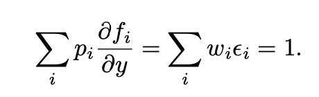
'adding up’ property of the cost function

the cost function is the sum of all (p*q) whereby q is obtained from the Hicksian

derive shepherd’s lemma from the cost function

taking the ‘adding up’ definition of cost

then, take derivative wrt price of good j = g(v,p) + SUM[ (p_i) dg/dpj ]

the p_i can be replaced with the Lagrangean FOC mu*du/dqi

which can be shown to make the second term equal zero

so dc/dp_j = g_j(v,p)

The derivative of the cost function wrt p is the Hicksian demand

Write the formula for roys identity and how can we derive it

-dv/dp_i / dv/dy = f_i(y,p)

Write the Lagrangian.

By Envelope Theorem, dL/dy = dv/dy = lambda

dL/dp = dv/dp = -lambda*q

Dividing the two equations yields our Roy’s identity result

how are indirect utility and cost functions related, mathematically

v(c(v,p), p) = v, whereby c(v,p) = y

c(v(y,p), p) = c

What is the Slutsky eqn for?

derive the Slutsky compensated eqn again

Slutsky relates the price effects on Marshallian with Hicksian.

First take the compensated demand fxn g, and differentiate wrt price

g = f(c(v,p),p)

dg/dp = df/dp + df/dc*dc/dp

dg/dp = df/dp + df/dy*dc/dp

dg/dp = df/dp + df/dy*(g(v(y,p) ,p)) ← Shepherds Lemma

dg/dp = df/dp + df/dy* (f(y,p)) ← equality of Hicksian/Marshallian

Hicksian demands - does it satisfy negativity? Why?

yes, satisfies negativity. this is because it is the derivative of the cost function. the cost function is concave in prices → implies negativity (substitution effect)

As long as WARP is satisfied

slutsky symmetry

by shepherd’s lemma, the two pairings gi/pj and gj/pi are both equal to each other in the slutsky eqn

dgi/dpj = dgj=dpi

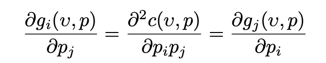
property of compensated cross-prices

the effect of increasing price i on good j is equal to the effect of increasing price j on good i

this is by the law of slutsky. complementarity and subsitutability are symmetric

which can only be applied to hicksian and not marshallian

adding up and the hicksian

sum of p*g = c(v,p)

homogeneity of marshallian

homogeneous of degree zero to price and income (doubling both leaves marshallian qty unchanged)

integrability

if demand functions:

• satisfy adding up

• homogeneity

• negativity

• symmetry

OR - the demand was derived from a utility maximisation / expenditure minimisation from convex ICs

OR - the demand was taken using shepherds lemma or roys identity

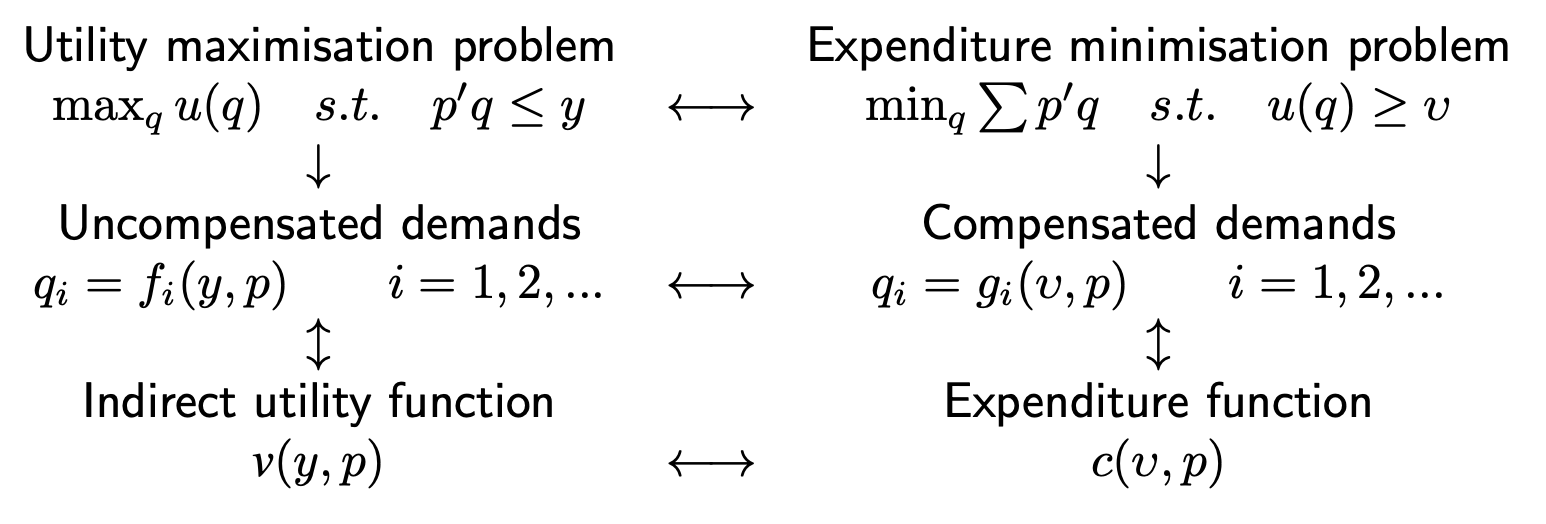
how do the utility maximisation problem, expenditure minimisation problem, marshallian demand, hicksian demand, indirect utility function and expenditure function all connect together?

diagram

homothetic preferences and impact on indices?

Homotheticity means that the cost function is v*f(p)

So it cancels out in the Konus.

Therefore the Konus is independent of utility (regardless of whether you’re rich or poor it affects you the same way)

change in consumer surplus - how is it found

‘lost’ area of the marshallian demand from old to new price (by integration)

compensated variation

expenditure function evaluated at the old utilities: whereby c(v0,p1) - c(v0,p0)

this is equivalent to the ‘lost’ area in the original Hicksian (at v0) where we integrate p0 to p1

equivalent variation

expenditure function evaluated at the new utilities: whereby c(v1,p1) - c(v1,p0)

this is equivalent to the ‘lost’ area in the new Hicksian (at v1) where we integrate p0 to p1

true cost of index

aka. T or Könus index

= c(v,p1) / c(v,p0)

when does the dependence on v disappear in the Könus index? what, then, is the value returned by the index?

what happens to KOnus if prices increase and preferences are homothetic?

when prices double, triple,etc. change by a common scalar

the index will return the scalar. (2 for doubling)

Konus scales proportional to the price change

Laspeyres index

L = sum(p1q0)/sum(p0q0)

evaluates quantity bundles at original prices

multiply by p0/p0 to get the alternate form: sum(w0 p1/p0)

Paasche index

P = sum(p1q1)/sum(p0q1)

evaluates quantity bundles at new prices

multiply by p1/p1 to get the alternate form: 1/sum(w1 p0/p1)

Envelope Theorem of cost function and indirect utility fxn

dC/dv = dL/dv = lambda

dC/dp = dL/dp = q (Hicksian)

dv/dy = dL/dy = lambda

dv/dp = - lambda * q1

Prove Roy’s identity

1. Use the Envelope Theorem to write out

dv/dy = lambda

dv/dp = -lambda*q

Divide 2nd by 1st eqn

net demand

z = q - w

where q is the gross demand (amount consumed)

w is the endowment

labour supply budget constraint

total value of consumption and leisure = full income (endowed income + total value of endowed time)

pc + wh = y + wT

substitution / income effect of price increase for…

1. demand without an endowment

2. demand with an endowment

3. labour supply

1. subs eff must be -. Inc eff generally - but if inferior good, will be + . Giffen good iff total effect is pos

2. subs eff must -, inc eff can be either + or - dep on buyer/seller

3. subs eff must +, inc eff must +, total eff is ambiguous

endowment income effect (define? and derive it please)

Definition: df/dY - MEASURES how changing endowment affects demand

Derivation:

1. Write out the equation for endowed demand. I.e. net demand = q - ω = φ

2. d(φ)/d(p) = ω(df/dY) + df/dp (By chain rule)

3. Using Slutsky’s eqn for df/dp, we get the required result: d(phi)/d(p) = dg/dp - z(dphi/dY)

where df/dY is our endowment income effect

steps for solving labour supply problems

1. replace c in the utility fxn with y+wL/p (this comes from the budget constraint pc=y+wL) and replace h with T-L

2. take FOCs wrt L and solve for L.

what are engel curves?

as income increases, what happens to demand and what happens to the share of expenditure

plots f against y, or w against y

tells you whether good is inferior or normal, or luxury/necessity

how do we find the final value of the Laspeyres or Paasche index?

1. Find the Marshallian demand

2. Using the formulas for Laspeyres or Paasche, plug in for q.

3. Simplify.

L or P should be functions of just p at the end (so you could plug in theoretical numbers and solve)

how do we solve Labour Supply questions?

1. Write down what we are trying to maximise and what the restrictions are. (Maximising utility fxn u(c,h), with restriction of c=y+wL)

2. Be sure to replace L with T-h. Remember that we want all h on the LHS and multiplied by its ‘cost’

3. Use MRS=MRT to find the optimal h

4. Find L

what is the only case where preferences are both homothetic and quasilinear? What is the form of the utility fxn in this case?

If the indifference map contains parallel straight lines to an axis.

This happens when goods are perfect substitutes. e.g. U(x,y) = ax+by

MRS & Homotheticity

• Can there be extra terms tacked on?

To check if preferences are homothetic, look at the MRS. It should be a function of only the ratio of q1 and q2. It does not matter if there are extra terms tacked on.

q1/q2 + 8 is homothetic.

Cobb-Douglas demand function shortcut

q₁ = (α/α+β)(y/p₁)

q₂ = (β/α+β)(y/p₂)

Along the income expansion path, the MRS is…

constant.

MRT does not change (budget set remains same) so the optimality condition MRS=MRT must hold. And so implies MRS is constant.

Homothetic preferences and budget share?

Regardless of income, the budget share of goods remains the same.

Quasilinear preferences (wrt good 1): what is the income elasticity for good 1? For good 2?

income elasticity for good 1 = 1

income elasticity for good 2 = 0

What is the only case in which there might be multiple solutions that solve optimality MRS = MRT?

If there are corner solutions. Which only happen if the budget set or indifference curves are not convex (one of the above)

how do we know if a demand is integrable (3 options to check)

1. derived from utility maximisation or cost minimisation from well-specified utility functions

2. derived from shepherds lemma or roy’s identity using well-specified functions

3. they satisfy negativity, adding up, symmetry, and homogeneity

What does SARP imply

In two good scenario, SARP implies WARP which implies negativity, homogeneity, and symmetry are met

compensating variation

the loss in CS integrating from p to p’ (following a price increase) evaluated at the initial level of utility

equivalence variation

the loss in CS integrating from p to p’ (following a price increase) evaluated at the final level of utility

Hicksian demand of a quasilinear good (wrt 1)

Only depends on prices of good 1. It does not depend on prices of good 2 nor the level of utility

How does the existence of endowments change the Marshallian? The Hicksian?

The Marshallian goes up beacuse the existence of endowments increases the budget set, so you can reach a higher utility.

The Hicksian stays the same. This is because you are still trying to minimise given a fixed utility.

Income and subsitution effect signs for labour supply

if an increase in w → increase in L what does this imply

what if increase in w → decrease in L?

are FLIPPED because it is a supply

for the demand of leisure, income eff must be + (leisure is a normal good), subs must be -

for the supply of labor, subs must be +, income eff can be -

s.t. an increase in w → increase in L implies the substitution effect dominates

if an increase in w → decrease in L this means income effect dominates

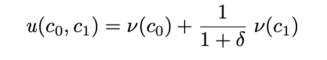
what does the utility fxn for a economy under intertemporality look like

there is a discount factor on the 2nd period

intertemporal elasticity of substitution (def?)

what does a higher elasticity imply

and how do we calculate it

measures how responsive the slope of IC is to changes in interest rate

dln(c1/c0) / dln(1+r)

higher elasticity implies more responsive, so the utility fxn is less concave

we calculate it from the FOC (MRT=MRS) where we can replace c1/c0 with y and 1+r with x

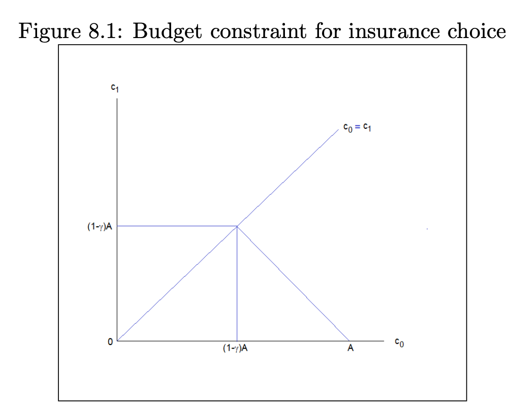
Derive the optimal conditions for the insurance choice problem and hence draw the budget constraint

good (no theft) c0 = A - Kp

bad (theft) c1 = K - Kp

A is wealth, K is amount insured, p is the premiums paid

Insurance / betting / tax-evasion problem. What variable do we eliminate to derive the budget constraint?

Eliminate the value that you want to know.

For example: insurance case eliminate the amount to insured

Betting eliminate the amount to bet

Tax-evasion eliminate the amount to evade

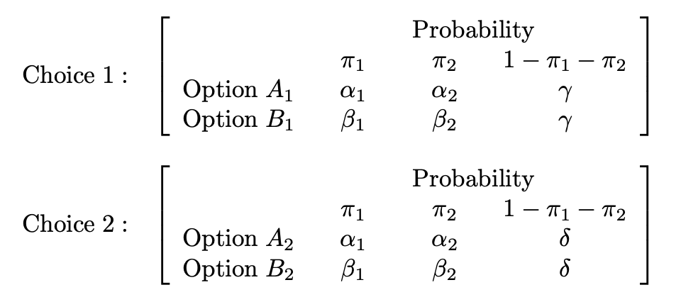
Sure thing principle

If there are two different lotteries with different payoffs corresponding to three possibilities, and lottery #1 is chosen,

Then in another case of two different lotteries with different payoffs, lottery #3 should be chosen. It is a case of induction.

How does risk aversion relate to the concavity of the utility function?

The more concave it is, the more risk averse the person is.

Actuarially fair

If the probability of getting into an accident (pi) is equal to the premiums paid (gamma), then the person will choose to insure the full wealth.

When does underinsurance happen?

If the insurance premium (gamma) is larger than the probability of getting into an accident (pi)

Allais paradox

Counterargument to the “Sure Thing Principle”

It shows from empirical evidence that this principle is violated, for example in the case of preferring certainty in one case (when there is a small chance of losing a lot) and preferring risk in another (when there is a small chance of gaining a lot)

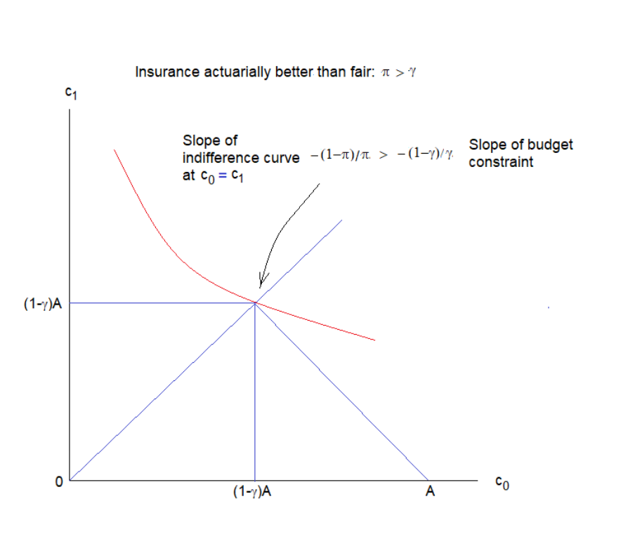
What if insurance conditions are better than fair?

Depends on the laws in the country. Assuming you cannot borrow money to buy more insurance then the point chosen is still full insurance, but utility is not maximised as there is an imaginary possibility of gaining more from borrowing and then purposefully choosing to be in the bad state.

Derive the optimal conditions for the betting problem and hence draw the budget constraint. Hint: Write out the expected utility.

good (win) c1 = (A-K) + K(1+r) = A+Kr

bad (lose) c0 = A - K

where A is your initial wealth, K is your bet, r is the return from winning

The expected utility function is…

E(U) = πv(c₁) + (1-π)v(c₀)

= πv(A+Kr) + (1-π)v(A-K)

Optimal conditions:

Take the derivative of E(U) wrt K and evaluate at K=0.

dE(U)/dK = πrv’(c₁) - (1-π)v’(c₀)

v’(A) [πr - (1-π)]

This marginal benefit must be larger than zero,

Hence: πr - (1-π) > 0, so πr > (1-π)

Derive the optimal conditions for the tax-evasion problem and hence draw the budget constraint

“good” (evade tax) c0 = Y - (T-D)

“bad” (get caught) c1 = Y - T - Df

D is amount of tax evaded

f is a fine paid on the amount of tax evaded

T is the amount of tax you’re meant to pay

Y is your income

income expansion path (draw an example)

• the path traced out by demands as y increases

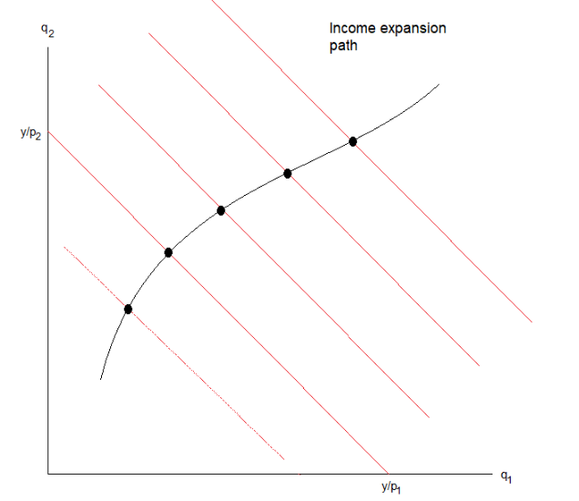
luxury

budget share of a good, w, rises with total budget

necessity

budget share of a good, w, falls with total budget

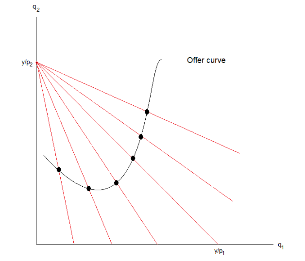
offer curve (draw an example)

the path traced out by demands as pi increases

Normal vs Giffen good (Tell me one thing abt Giffen goods and the Slutsky)

Own price elasticity - when it is negative it is a normal good. When it is positive it is a Giffen good

Giffen goods - the income effect dominates the substitution effect in the Slutsky

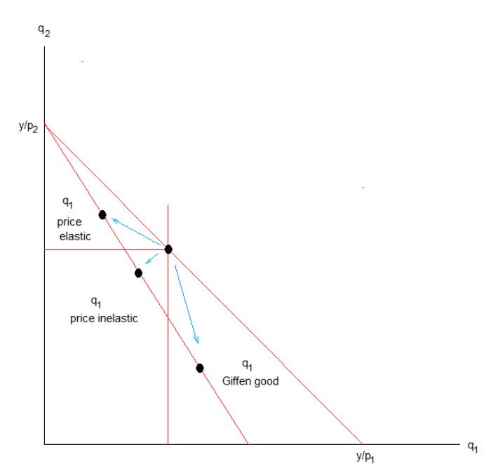
Price elastic good (Draw an example of price increase and price elastic good)

The own-price elasticity is less than -1. If budget share falls with price

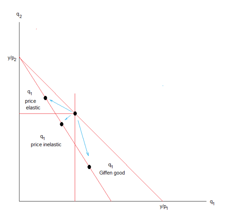
Price inelastic good (Draw an example of price increase and price elastic good)

The own-price elasticity is between -1 and 0. If budget share rises with price.

Cross price elasticity. Sign for complement/substitute?

Positive sign - substitute

Negative sign - complement

Engel aggregation (Derive)

What does the Engel aggregation imply?

Differentiate adding up wrt y

Rewrite as product of wage share and income elasticity by multiplying (y/q)(q/y)

Implies

1. Not all goods can be luxuries

2. Not all goods can be necessities

3. Not all goods can be inferior

Cournot aggregation (No need to derive, just state the implications)

Implies that when price of one good increases then purchases of some good (not necessarily that good) must DECREASE

WARP definition?

Weak axiom of revealed preferences

If bundle Qa is chosen when Qb is affordable, then Qb should never be chosen when Qa is cheaper

In the two good scenario, SARP violation implies…

WARP is violated

In the three or more good scenario … a violation of SARP implies…

Does not imply directly that WARP has been violated. SARP is stronger than WARP so if SARP is violated this doesn’t prove that WARP is violated. If however WARP is violated then yes SARP is violated

Law of Demand from Slutsky

If a good is shown to be normal, then df/dp must be negative if dg/dp is negative (→ dg/dp is always negative by negativity which only requires WARP)

Giffen Goods (Demand curve? WARP? When do we get them? INtuition?)

Demand curve is upward sloping

WARP satisfied

We get them even when the income effect is so strong that it dominates the substitution effect.

Intuition: Very poor communities where the price increase effectively restricts their consumption to just that inferior necessity good, forcing them to consume more of it (e.g. no longer able to afford meat, so they consume more rice)

IBC for intertemporal question (assume income y, assume no endowments nor profits)

c₁ = (y₀-c₀)(1+r)+y₁ if savings earn interest

c₁ = y₀ + y₁ - c₀(1+r) if savings dont earn interest

General eqbm definition

how is this diff from walras’ law

Z_i = Sum(z_i^h) = 0

Where z_i^h is the excess demand of good i for household h.

Z_i is the excess demand of good i for all households.

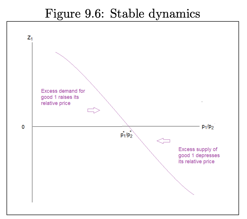
walras’ law: the value of agg. excess demand is zero. (Sum pZ = 0)

Walras’ Law (intuition? formula? what does it imply? and in the two-good mkt?)

Intuition: price*Aggregate demand equals price*Aggregate endowments. And so price*Aggregate excess demand = 0

→ Sum(p_i*Z_i) = 0 follows from aggregate excess demand times price = 0.

Implies there are only M − 1 independent equations determining M − 1 relative prices. Where M is the total number of goods.

Hence in the two-good mkt, general eqbm of one good (Z_i = 0) implies the other good is also in eqbm (Z_j = 0)

Draw the stable dynamics graph, relating relative price to excess demand.

When there is excess supply, what must happen to reach equilibrium?

weakly preferred set (State the name of this set) of bundle q^A

The upper contour set “R”

All bundles of q^B which q^B >~ q^A

qB is at least as good as qA

weakly dispreferred set (State the name of this set) of bundle q^A

The lower contour set “L”

All bundles of q^B which q^A >~ q^B

qA is at least as good as qB

indifference set of q^A

• intersection of both “R” (Upper) and “L” (Lower) contour sets

• all bundles of q^B s.t. q^B ~ q^A

Completeness (Definition? How does it look visually on a map of q1 and q2)

There is no scenario where the consumer is unable to decide and does nothing. They either prefer one bundle over the other, or are indifferent between bundles.

In the map: Completeness means the sets L and R cover the whole space of the map (With the intersection being the indifference set)

Transitivity?

Draw an example of violation of transitivity side-by-side to adherence of transitivity

What’s a common preference criterion that violates transitivity?

Revealment of indirect preferences must hold. If qA >~ qB and qB >~ qC then it must be that qA >~ qC or else there will be a cycle

qA>~qB if qA1 > qB1 or qA2 > qB2 (Draw it out. Then a bundle qB that has more of good 1 but less of good 2 is both preferred and dispreferred to qA, which does not make sense. → a cycle)

Preference ordering requires what conditions to hold?

• Transitivity

• Completeness

Nonsatiation

No bliss points

→ You can always move to a point that makes consumer better off

Monotonicity

ICs slope down, s.t. MRS is always negative

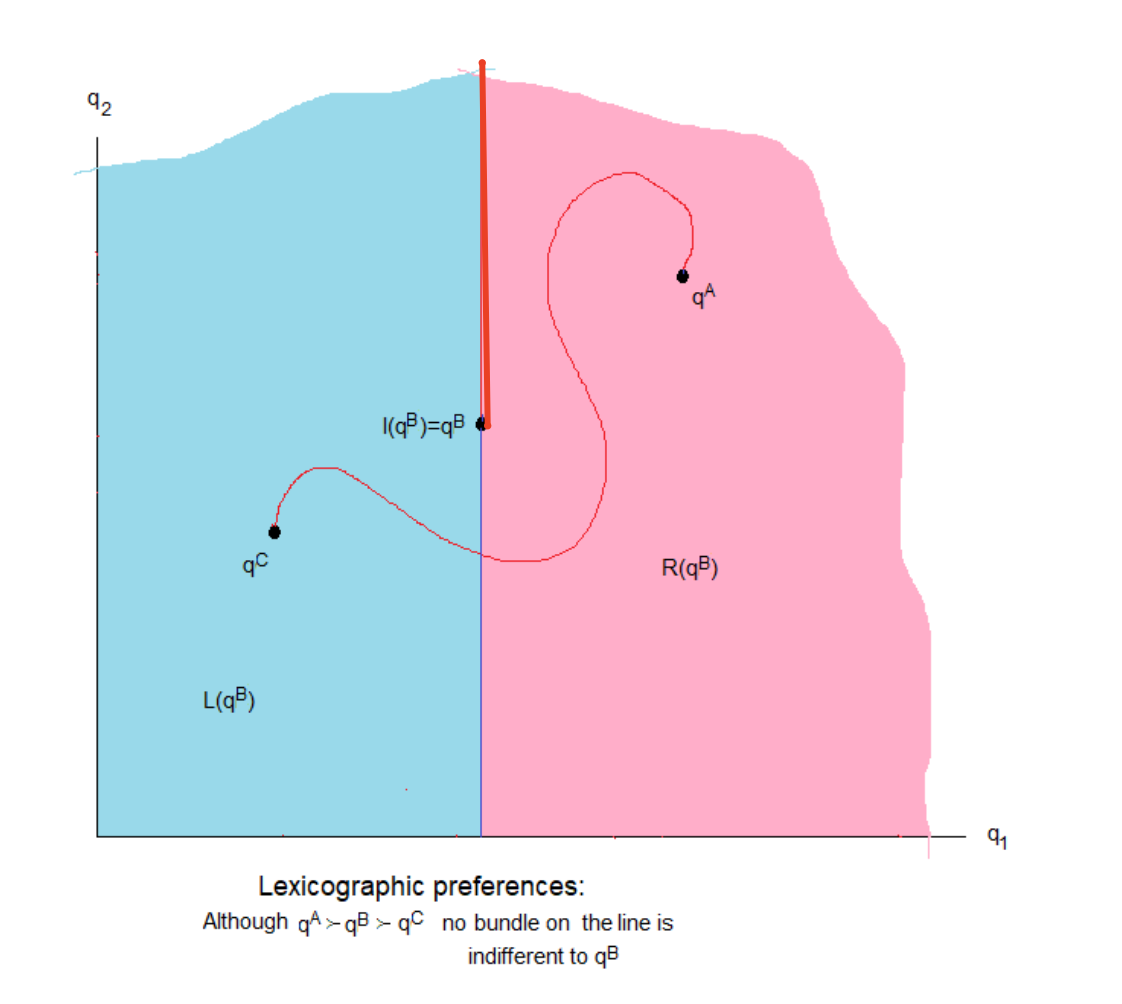
lexicographical preferences

(What does it violate)

qA >~ qB

If:

• qA1 > qB1

OR

• qA1 = qB1 and qA2 > qB2

Violates continuity because you can draw a line from A to C without crossing the indifference set of B.

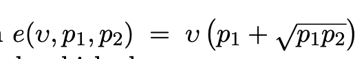
how to detect homotheticity given a cost function?

the utility in the cost function is multiplicative of a function of price

v*f(p)

example

how to detect luxury/necessity given a cost function

find the Hicksian, then find the budget share and see if it is increasing or decreasing in utility

SUPPOSE that bundle A is revealed directly preferred to B

yet bundle B is simultaneously revealed directly preferred to A

what preference rule does this violate?

transitivity

when might a consumer choose to consume none of a good, despite regular utility fxn

explain.

if quasilinear, wrt to good 1,

then if the budget is too low, then consumption of good 1 will be zero.

this comes from the fact that q2’s marshallian demand is always a fxn of just p, which is always positive. but q1 depends on y. so q1 may not always be positive.

Eqbm in production economies

What is the individual budget constraint?

Each firm tries to maximise profits = y^kp^’ = P*F(L) - w*L

Each individual owns a percent of the profits, theta. Sum of all theta = 1.

The individual budg constraint: p’q^h = p’w^h + sum_ktheta^hk(p’y^k)