L7 Vision Transformers

Visual tokenization

The process of converting image data into sequences of discrete tokens suitable for transformers. Unlike traditional CNNs, which process images in a spatially-aware, hierarchical manner, visual tokenization treats images as a sequence.

Steps:

1. Patching

2. Patch embedding

3. Quantization (optional)

4. Positional encoding

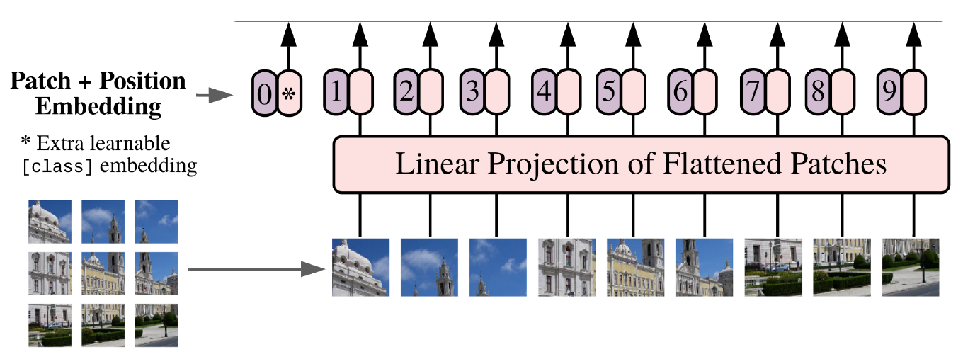
Patch embedding techniques

• Learned linear projection layer (after flattening the patches) → uniform for each patch

• Fixed CNN-backbone

Positional embedding types

• learned (e.g. embedding layer)

• fixed (e.g. sine/cosine)

Positional encoding in ViTs

CNNs inherently capture spatial relationships via local receptive fields, while transformers rely on positional encodings to recreate this spatial structure.

Types:

• additive: e^patch + e^pos(x,y) → the absolute position is used

• relative: depends on the distance between the query’s and key’s position in the sequence, instead of absolute positions → calculated in each attention layer

• bias: a learned bias term is added to the attention scores. Sometimes two-phase attention is used, first with (Q, e^rel , V), the results of this are used as a bias in the original (Q, K, V) attention.

ViT Architecture

Vision Transformers (ViT) process images as a sequence of patches, embedding each patch, and passing these embeddings through transformer layers, traditionally designed for NLP tasks.

Unlike CNNs, ViT does not rely on convolutions, allowing it to leverage self-attention mechanisms to model global relationships more directly.

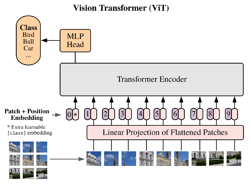
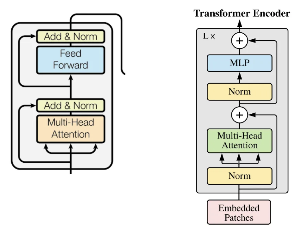
Difference between ViT’s encoder and normal transformer encoder

Normalization comes before the first layer, not after = pre-normalized transformer encoder -> adds extra regulation

2. MLP head added: only uses the first element of the sequence, which has the role of aggregating all the inputs which are needed for the classification

Classification token in ViT

A dedicated token added to patch embeddings in ViT, which has the role of aggregating all the inputs which are needed for the classification, therefore learning a global representation for the entire image. During inference, the transformer output for this token is passed to the MLP head for classification.

=> In CNNs, global representations are achieved through pooling layers, but ViT’s CLS token offers a more flexible, learnable representation.

Higher Resolution Processing in ViTs

Adapting the transformer architecture to handle larger image resolutions, allowing the model to capture finer details by processing longer sequences of image patches.

Only the positional encoding is dependent on size → we can interpolate the pre-trained positional encoding values to get more points for a longer input

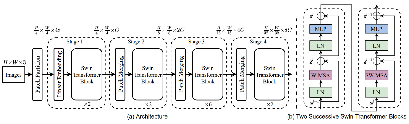
SWIN transformer

• able to process images of arbitrary size using a hierarchical design of multiple resolution levels

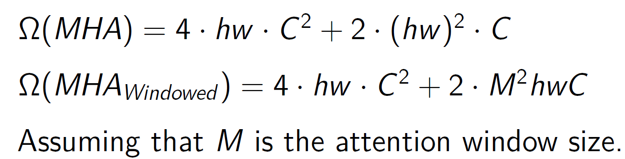
• local attention: limited to non-overlapping windows

• introduces a window-shifting mechanism for information flow across distant regions

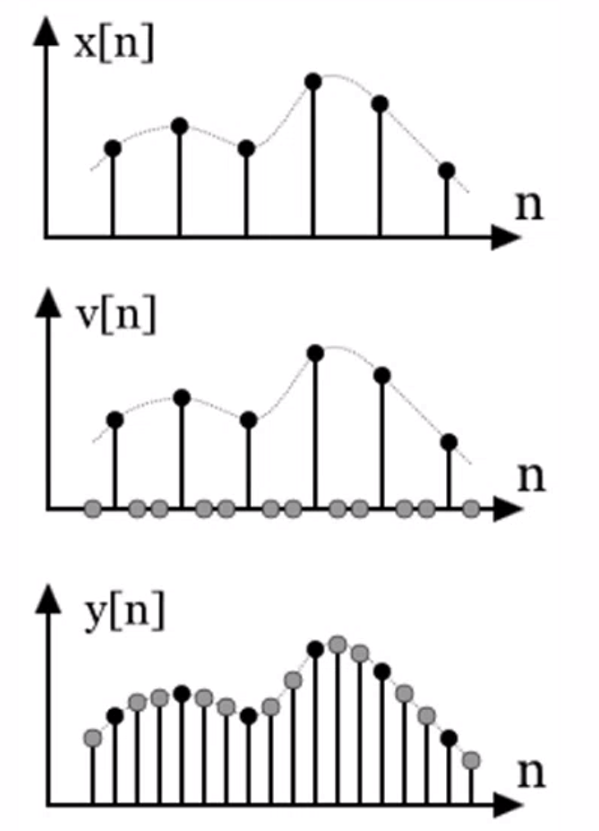
• tokens are merged (pooled) by a learnable projection at each level

Advantage of SWIN over ViT

Dramatically reduces computational complexity from quadratic to linear with respect to image size

→ more scalable to high-resolution images

→ widely used for semantic segmentation and object detection

Window shifting in SWIN

Shifting attention windows in consecutive layers in a cyclic manner, enabling interactions between adjacent windows and allowing information to propagate across the entire image.

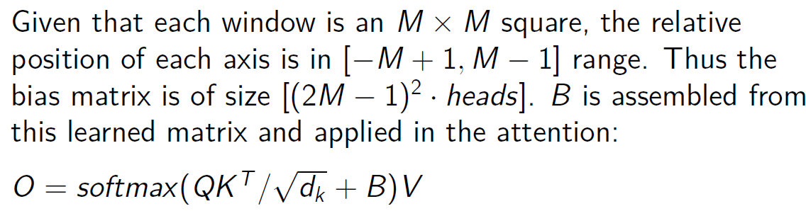
Learnable relative attention bias in SWIN

• a bias term is learned for each possible relative position of two tokens within the window
  → (2M-1)² bias for each head

• the bias corresponding to the current query and key is added to the attention score

• adapts well to different input sizes and can generalize better across various resolutions

• ←→ Requires additional training to learn optimal bias terms for each window

Knowledge distillation

A training technique where a smaller model (the student) is trained to mimic the outputs of a larger, pre-trained model (the teacher), often by using the teacher’s “soft” probability distributions instead of hard labels.

Advantages:

• smaller, more efficient models with faster inference

• can transfer performance from large, complex models to simpler models

Disadvantages:

• The student model’s performance is limited by the quality of the teacher

• distillation doesn’t always generalize well to significantly smaller models.

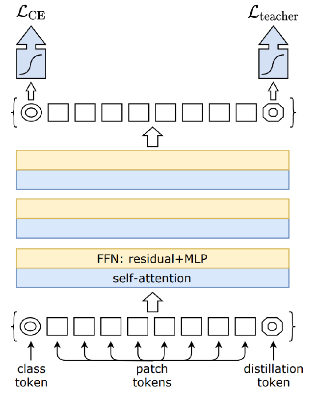
DEIT

= Data Efficient Image Transformer

A ViT variant that incorporates a distillation token in the input sequence as well

→ learns from a teacher model by optimizing the mean of the classification and distillation loss (cross-entropy of the ε-smoothed hard teacher and student logits)

→ the teacher’s prediction is set to 1 − ε, and the rest of the probability mass is distributed among the other classes to get soft labels

→ during inference, the dist. and class. logits are summed before softmax

Use Cases: Applied in scenarios where training data is limited but high-quality CNN models are available for transfer learning.

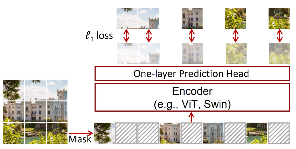
SimMIM

= Simple Masked Image Modeling

• A self-supervised pre-training approach similar to BERT in NLP

• random image patches are masked, and the model is trained to reconstruct the missing parts using a MASK token

• L1 loss between predicted and ground-truth patches is used

=> Improves feature learning, reduces model “data hunger,” and enables pre-trained ViTs to generalize well across downstream tasks.

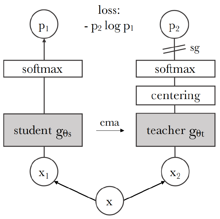
DINO

= self-DIstillation with NO labels

• Aims to find representations which are stable in the dataset

• Leverages self-distillation without labels by using an exponential moving average-based teacher model derived from the student’s past states.

• The teacher predictions are mean-centered and sharpened, guiding the student to learn stable and informative features.

• Optimizes cross-entropy between the student and

  the slowly evolving teacher

DINOv2

Masked modeling is added (only to student), along with data curation

=> achieves extremely good image embeddings

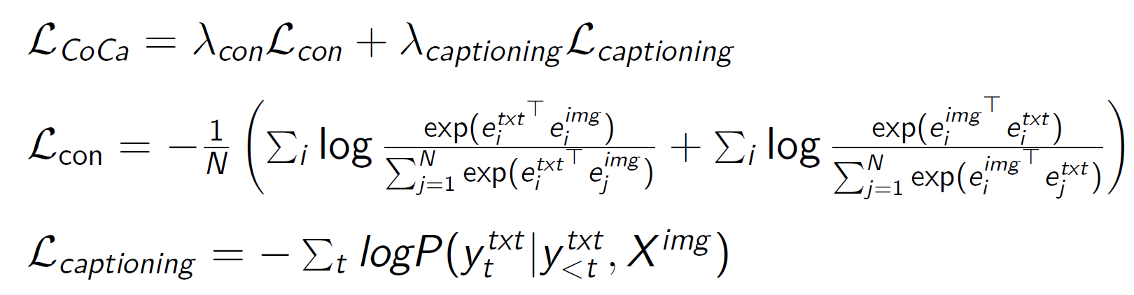
CoCA

= Contrastive Captioners

• a multi-modal model

• embeds images and text into a joint embedding space for contrastive learning

• the model can use both modalities for few-shot learning and retrieval tasks → e.g. image captioning or based on a text prompt finding the most relevant images from a database

• the image encoder is run only once, while the text decoders are run for each generated token

• The image encodings serve as the keys and values, while the unimodal text decoder’s current output is the query

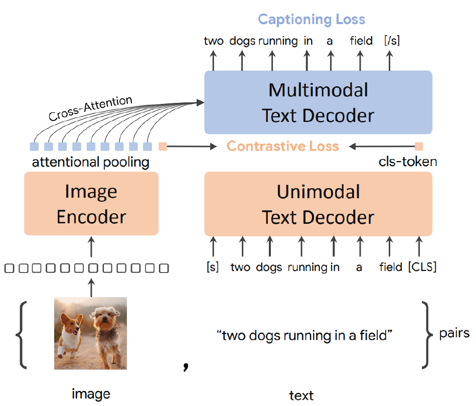
CoCA training

1. Encoder pre-training (supervised classification)

2. Simultaneous contrastive and reconstruction training

• Contrastive training to match pooled image embedding and CLS token from text representation (pair-wise dot-product similarity)

• Reconstruction training to reconstruct the original caption from the encoded image (autoregressive text prediction, using all image embeddings and all text embeddings generated so far)

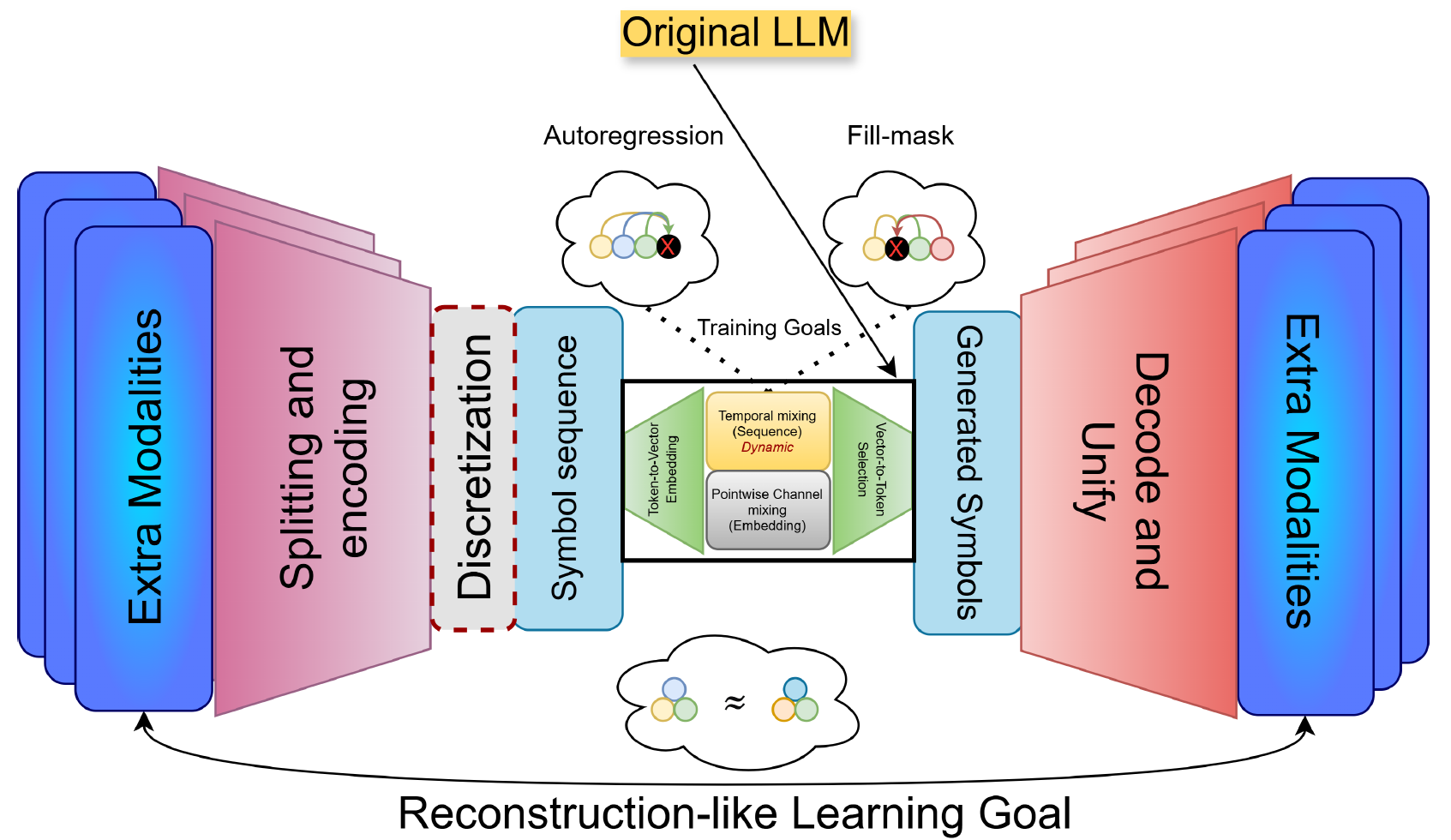
Large World Models

These models aim to learn generative representations across multiple modalities (e.g., text, image, video), creating a comprehensive model of the world, which can generalize across tasks and domains.

Recipe for Large World Models

1. Train a tokenizer (Encoder-Decoder model)

2. Train a transformer with Masked Modeling or Predict Next Token task in the latent space of the VAE.

3. For multiple modalities train multiple VAEs and require the single transformer to indicate output modality.

4. Use the corresponding encoder and decoder for each modality in the sequence.

Why might discrete latent spaces be beneficial over continuous ones?

Discrete latent spaces enforce a bottleneck that can lead to more meaningful, structured, compact representations.

• Compact, efficient code.

• Easy autoregressive modeling (discrete code acts as tokens)

• Interpretability.

• Reduces posterior collapse.

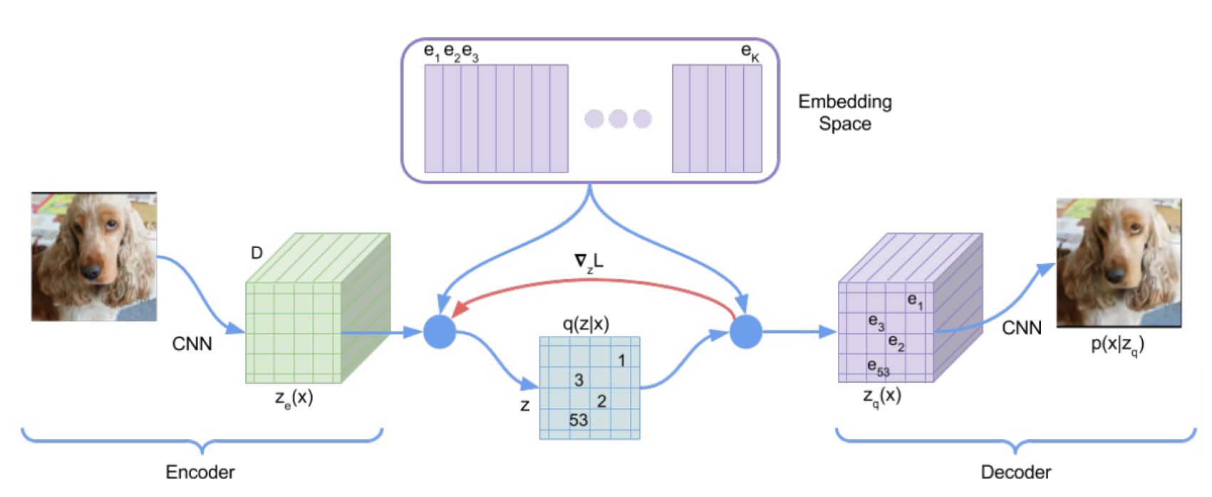
VQ-VAE (Vector Quantized VAE)

• encodes the input into a discrete latent space

• uses hard quantization: assigns each embedded input vector to the nearest vector from a fixed codebook

• decodes from the assigned codebook vectors

(It's called variational because it models discrete latent variables with approximate inference, using quantization as a discrete bottleneck instead of a continuous distribution.)

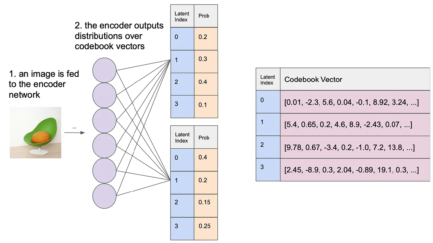
dVAE (discrete VAE)

• a type of autoencoder that represents input data in a discrete latent space

• Unlike continuous VAEs, dVAE reduces the continuous latent space to discrete units = greedily samples from a distribution

• => enhances interpretability and enables tokenization for transformer processing ←→ may loose detail

Unlike VQ-VAE, this does not encode the input into a latent representation, it encodes it into a distribution over the codebook for each position ( Instead of outputting a continuous vector in latent space, it outputs a soft distribution over discrete codes.)

Then during training, it samples from this distribution to get a stochastic representation for that position, and then decode from them

<-> during inference, it typically chooses the codebook vector with the highest probability for deterministic encoding

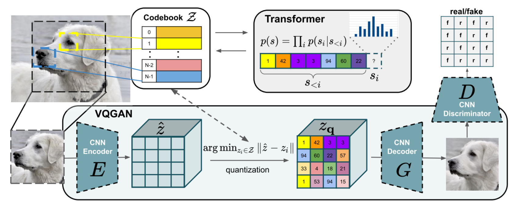
VQ-GAN

• combines the principles of vector quantization and adversarial training

• the generator is a VQ-VAE => the discriminator ensures the creation of an efficient codebook

• compared to VQ-VAE, in addition to reconstruction loss, this model includes a perceptual loss → ensures that generated images are not only visually accurate but also perceptually similar to real images.

Advantages:

• creates sharper images (VQ-VAE’s output is often blurry)

• perceptual loss ensures semantic consistency