week 4 pt 2 - unsupervised learning

supervised learning

labelled observations - pairs of data points, each pair consists of a feature vector (x) + its corresponding output label (y) which are related according to an unknown function f(x) = y

• during training- use these pairs to learn the relationship between x+y i.e. find a function (or model) h(x) that best fits the observations

goal = ensure that the learned model h(x) accurately predicts the output label of a previously unseen, test feature input (generalisation)

• labels = ‘teachers’ during training + ‘validator’ of results during testing

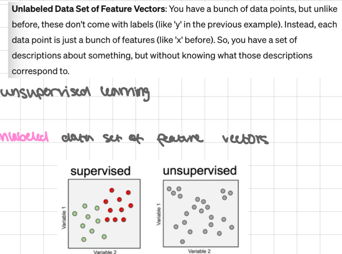
unsupervised learning

unlabelled data set of feature vectors

what can we deduce?

• even without labels, can still learn some interesting stuff from this data:

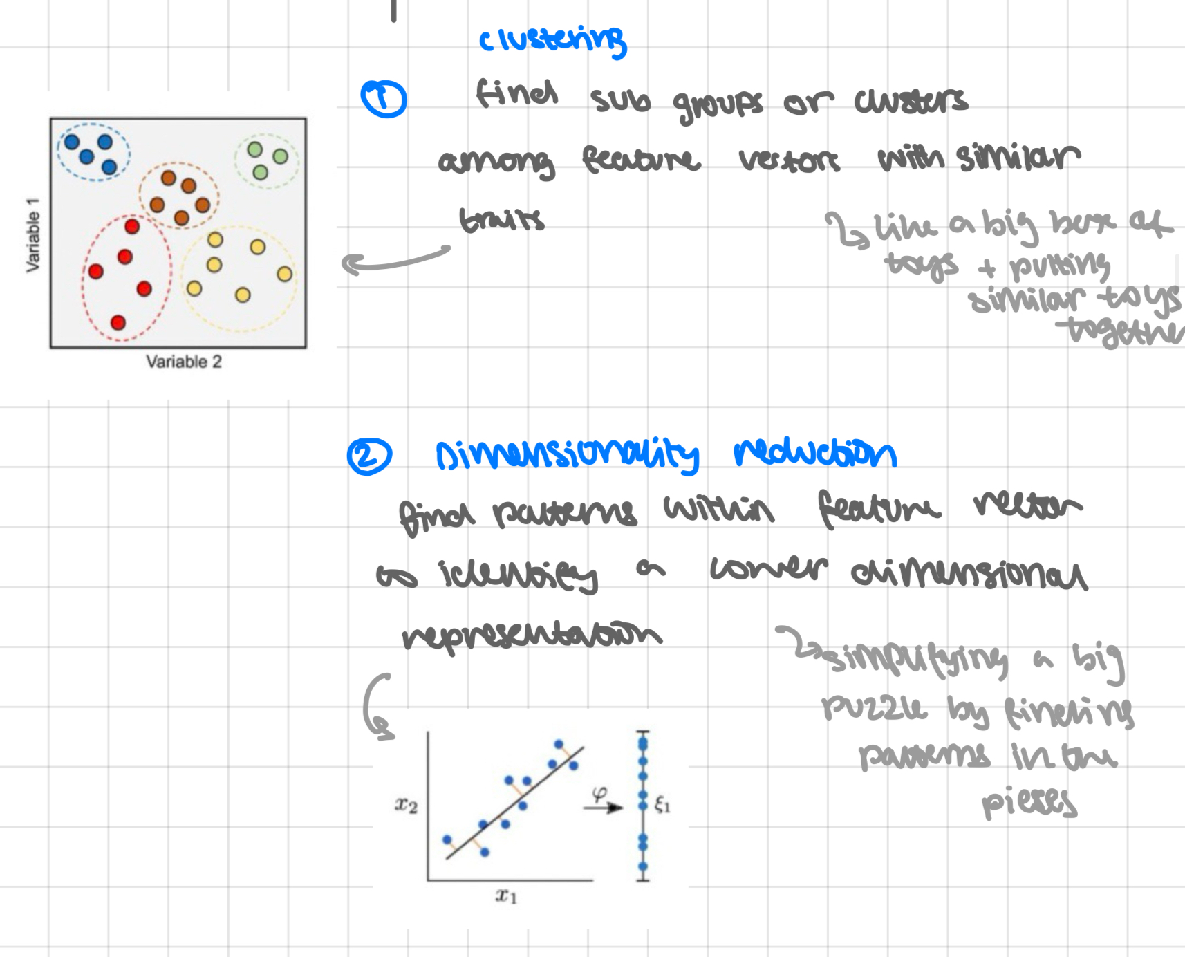
  1. clustering find sub groups or clusters among feature vectors with similar traits

     • like a big box of toys + putting similar toys together

  2. dimensionality reduction find patterns within feature vector to identify a lower dimensional representation

     • simplifying a big puzzle by finding patters on the pieces

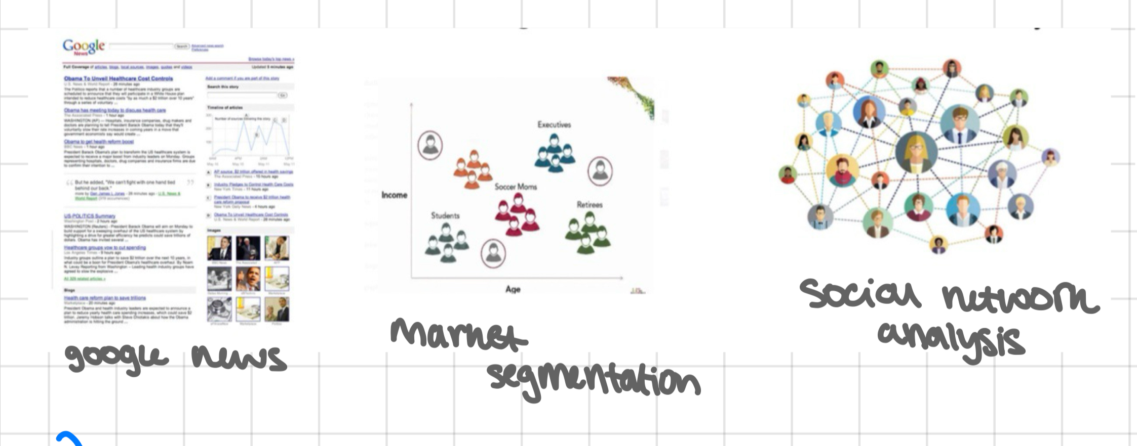
CLUSTERING - real world applications

google news

market segmentation

social network analysis

• clusters = potential ‘classes’; clustering algorithms automatically find ‘classes’

DIMENSIONALITY REDUCTION - application

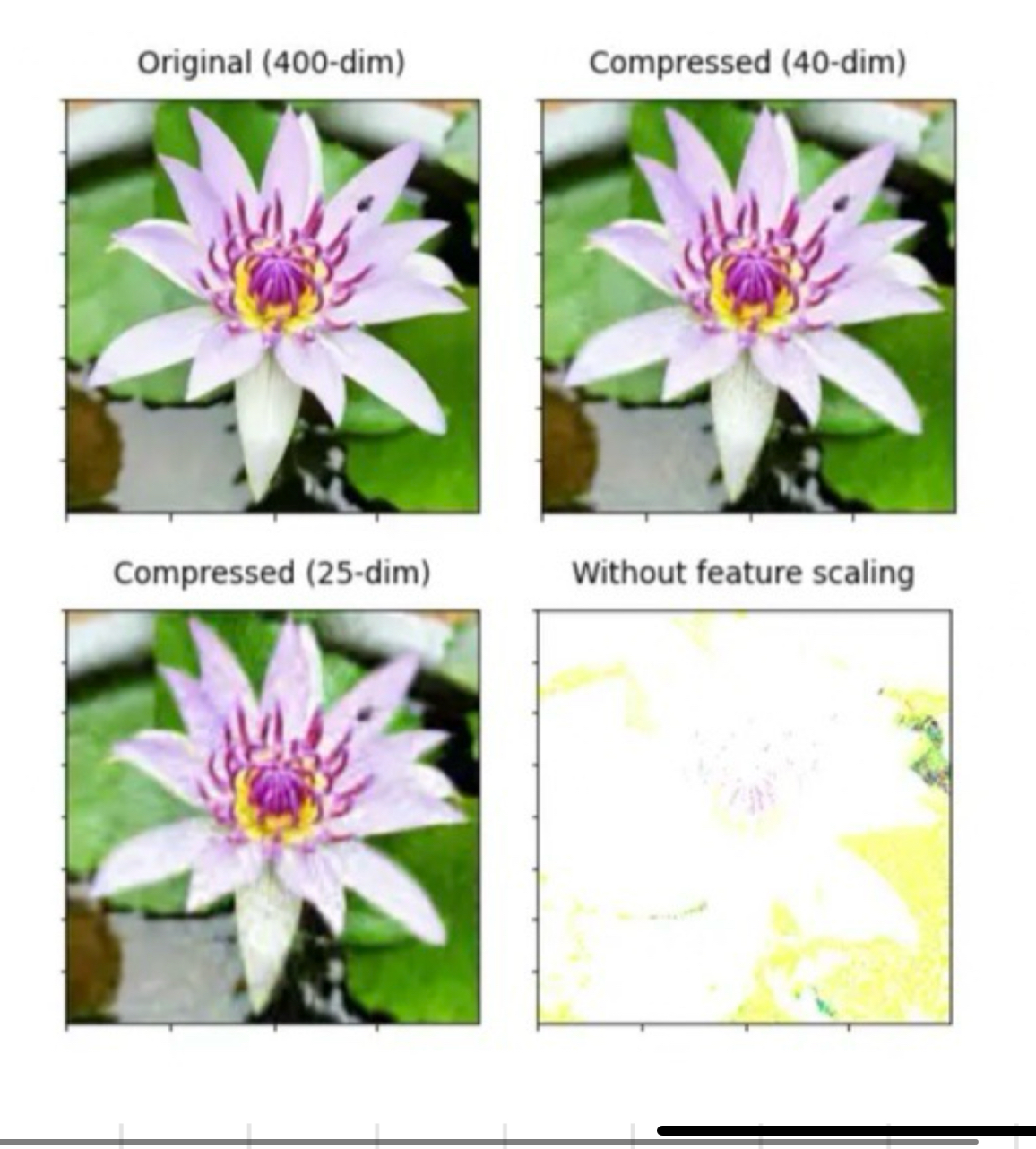
image compression

techniques:

• principal component analysis - finds main themes in data

• non negative matrix factorisation - breaks down complex mixtures

• linear discriminant analysis - helps you desperate diff groups based on their features

why unsupervised learning?

• labelled data = £££ + difficult to collect - unlabelled = cheap + abundant

• compressed representation - saves on storage + computation

• reduce noise, irrelevant attributes in high dimensional data

• pre processing step for supervised learning

• often used more in exploratory data analysis

challenges in unsupervised learning

• no simple goal as in supervised learning

• validation of results is subjective

fundamentals of clustering

goal: find natural groupings among observations/objects/feature vectors

segment observations into clusters/groups such that:

• objects within a cluster have high similarity (high intra-cluster similarity)

• objects across a cluster have low similarity (low intra-cluster similarity)

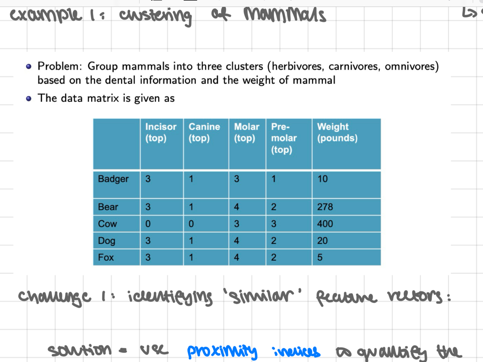
example 1: clustering of mammals

challenge 1: identifying ‘similar’ feature vectors:

solution = use proximity indices to quantify the strength of a relationship between any 2 feature vectors

depends on data type:

• continuous valued feature attributes

  • e.g. x = (0.1, 11.65, 15, 1.4)

• nominal feature attributes

  • e.g. x = (‘large’, ‘medium’, ‘small’)

  • must be mapped to discrete values consistently e.g. ‘large’ → 3, ‘medium’ → 2, ‘small’ → 1

continued

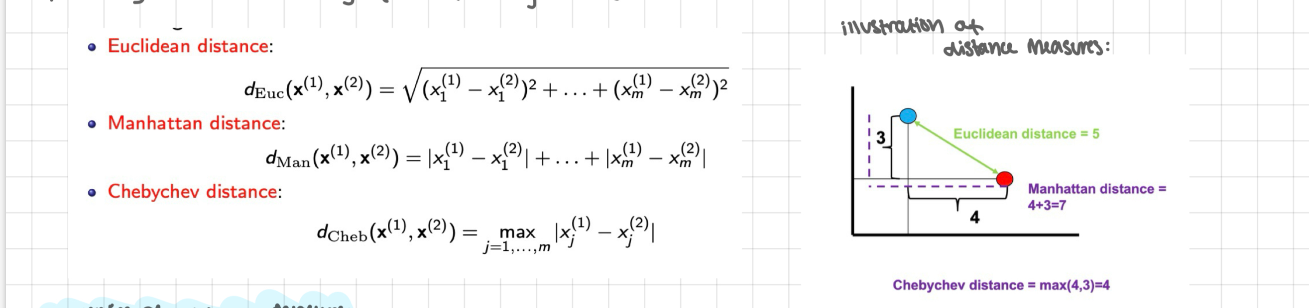
1. continuous valued features: for 2 continuous valued features x⁽¹⁾ = (x⁽¹⁾, …, x⁽¹⁾_m) and x⁽²⁾ = (x⁽²⁾, …, x⁽²⁾_m), the proximity index can be any of the following distances

   • euclidean distance

   • Manhattan distance

   • chebychev distance

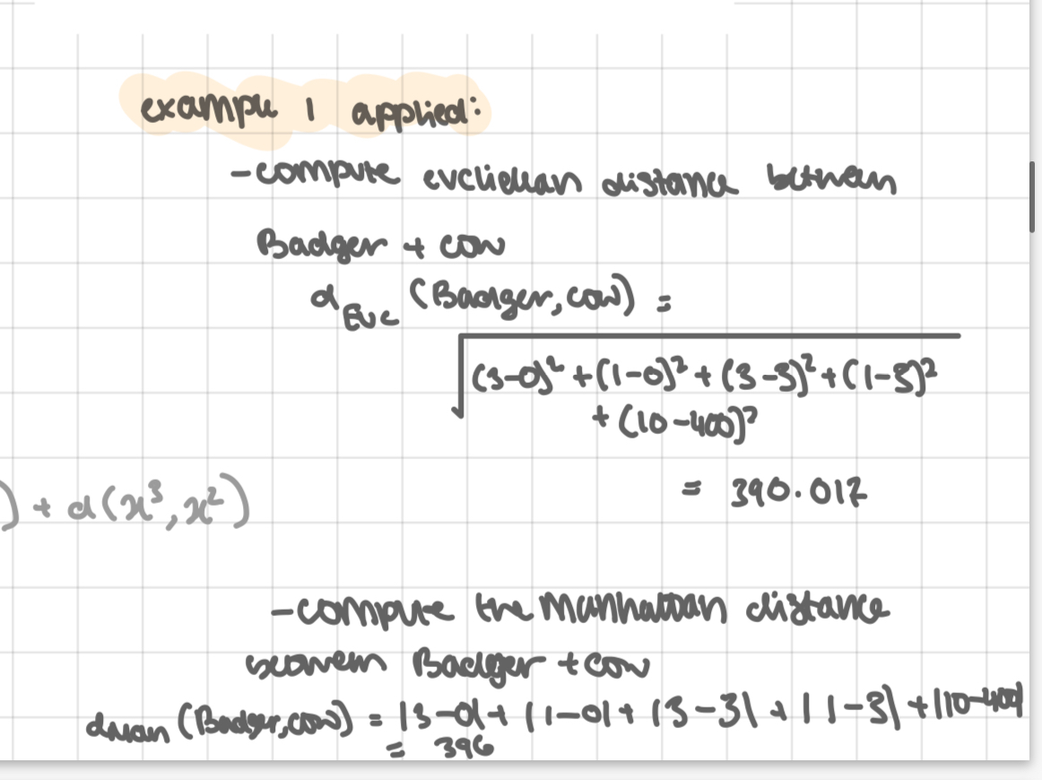
example 1 applied: see pic

continued pt 2

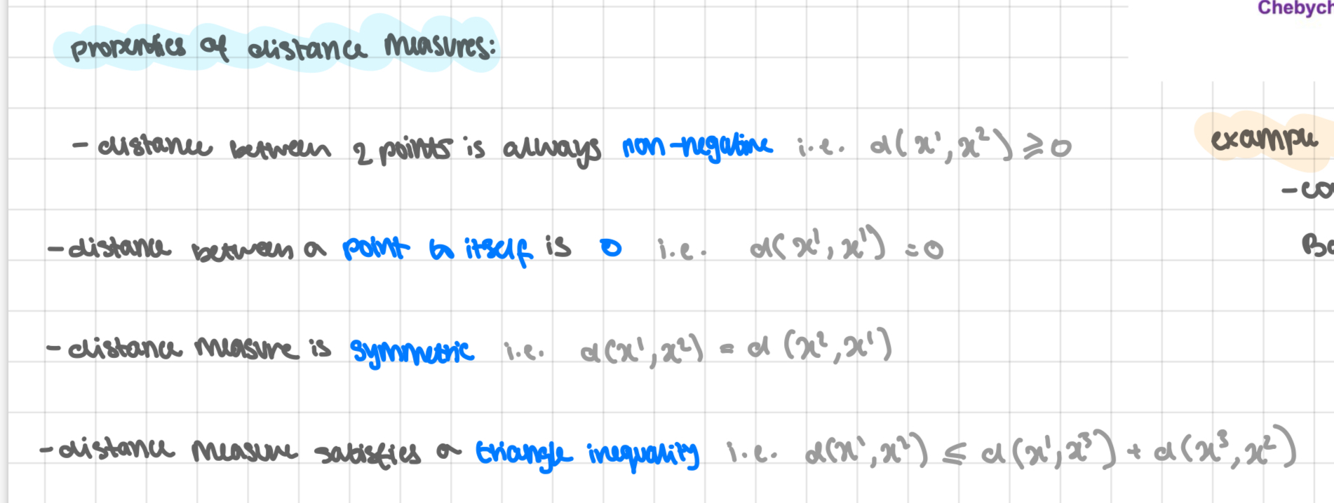
properties of distance measures:

• distance between 2 points is always non negative

• distance between a point to itself is 0

• distance measure is symmetric

• distance measure satisfies a triangle inequality

main takeaways:

- diff choice of distance functions yields diff measures of similarity

- distance measures implicitly assign more weighting to features with large ranges than those with small ranges

- rule of thumb: when x prior domain knowledge → clustering should follow the principle of equal weighting to each attribute

• this necessitates feature scaling of vectors

challenge 2: feature scaling

when feature attributes have large differences in the range of values, scaling of features = essential - so that each attribute contributes equally to the distance feature

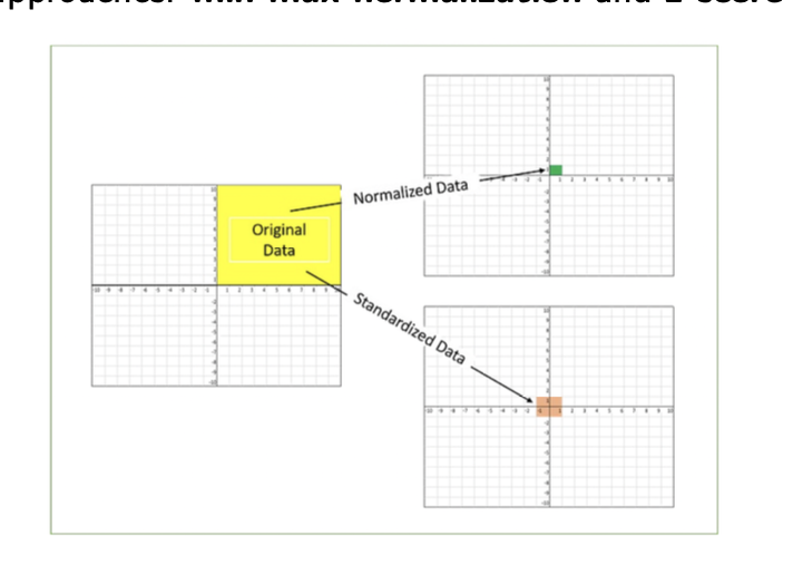
2 well studied approaches:

1. min-max normalisation

2. z score standardisation

minimum maximum normalisation

all feature attributes are rescaled to lie in the [0, 1] range

steps:

1. consider N feature vectors x⁽¹⁾ = (x⁽¹⁾, …, x⁽¹⁾_m), x⁽²⁾ = (x⁽²⁾, …, x⁽²⁾_m), x^(N) = (x^(N), …, x^(N)_m)

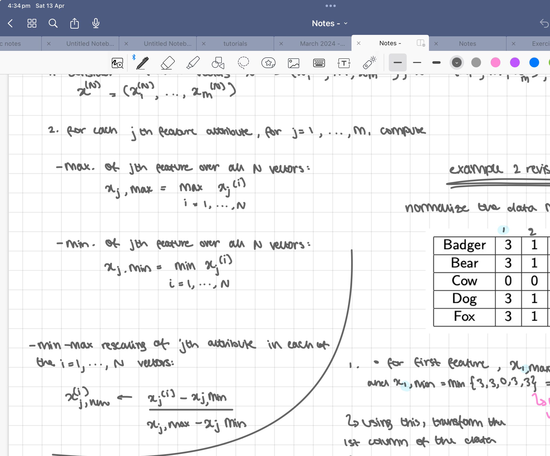
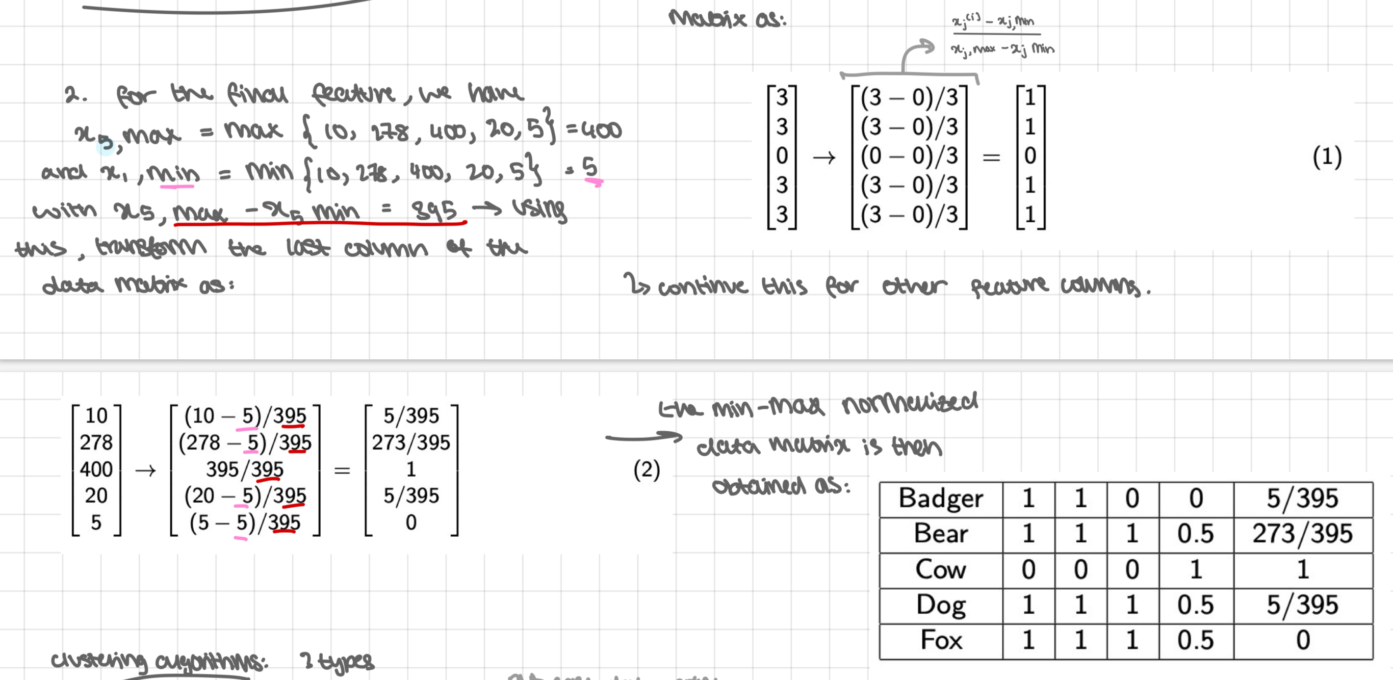
2. for each jth feature attribute, for j = 1, … m, compute

   • max. of jth feature over all N vectors:

     x_j,max = max x_j⁽ⁱ⁾ i = 1,…,N

   • min. of jth feature over all N vectors:

     x_j,min = min x_j⁽ⁱ⁾ i = 1,…,N

   • min-max rescaling of jth attribute in each of the i = 1, …, N vectors:

     x⁽ⁱ⁾_{j, new = (}x_j⁽ⁱ⁾ - x_j⁽ⁱ⁾min)/ (x_j⁽ⁱ⁾max - x_j⁽ⁱ⁾min)

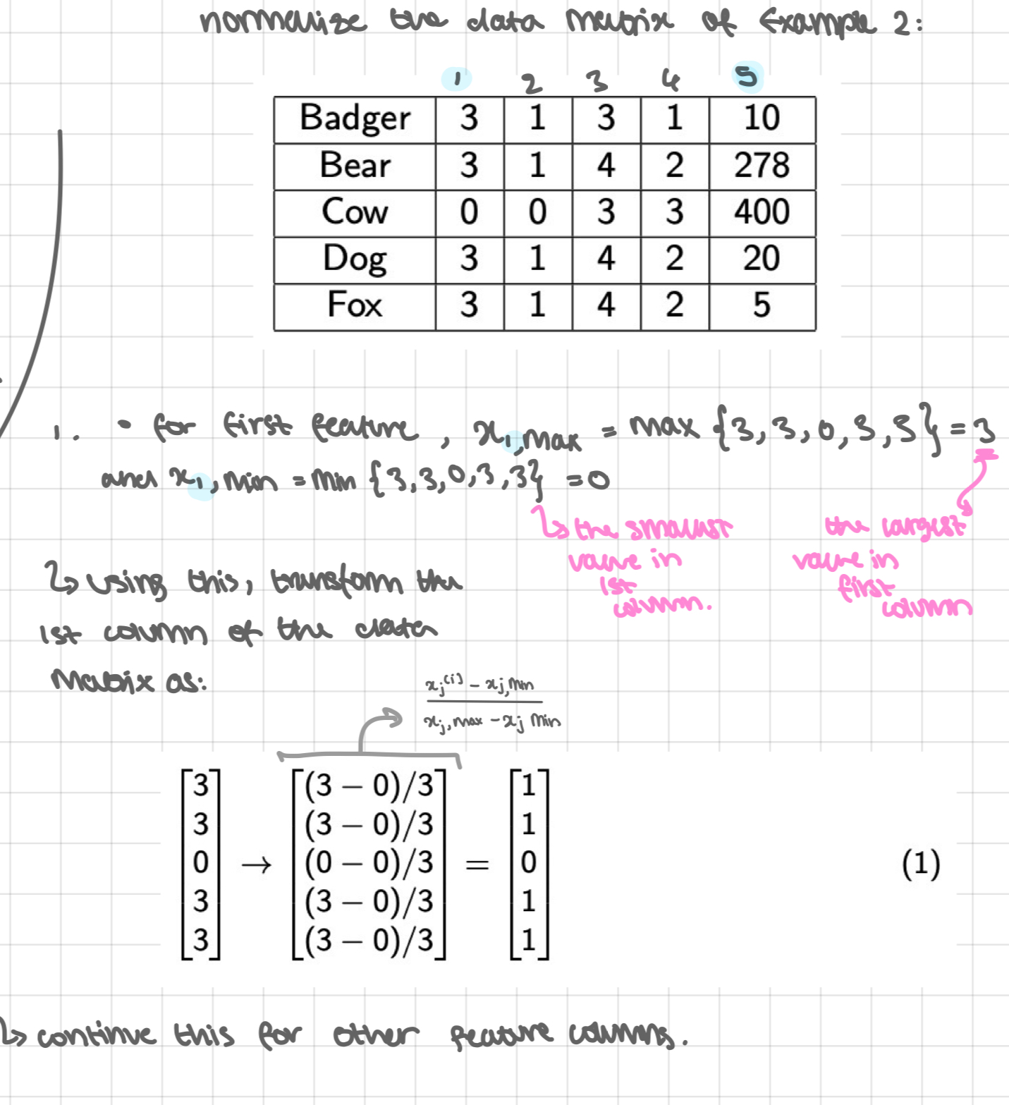
example 2 revisited: normalisation

CLUSTERING ALGORITHMS: 3 types

→ PARTITIONAL CLUSTERING ALGORITHMS

• generate a single partition of the data to recover natural clusters

• input: feature vectors

• examples: k-means, k-medoids

  • put each data point into 1 group or another based on certain characteristics they share

→ HIERACHICAL CLUSTERING ALGORITHMS

• generates a sequence of nested partitions

• input: distance matrix, which summarises the distances between diff feature vectors

• example: agglomerative clustering, divisive clustering

  • instead of just 1 partition, they generate a sequence of nested partitions = organise data points into clusters within clusters

→ MODEL-BASED CLUSTERING ALGORITHMS

• assumes that the data is generated independently + identically distributed from a mixture of distributions, each of which determines a diff cluster

• example: Expectation-Maximisation (EM)

partitional clustering algorithms: the basics

goal: assign N observations into k clusters, where k<N that ensure high intra cluster similarity + low cluster similarity

• high = clusters are v close

• low = clusters are v. far

can be formulated as a combinational optimisation problem* = requires defining a measure of intra-cluster similarity

• where we search for the best arrangement of clusters among all possible arrangements

Notation:

• C denote a clustering structure with K clusters

• c ∈ C denote a component cluster in the clustering structure C

• e ∈ c denote an example in cluster c

measuring intra-cluster similarity

like a ruler to see how close or similar things are within a cluster

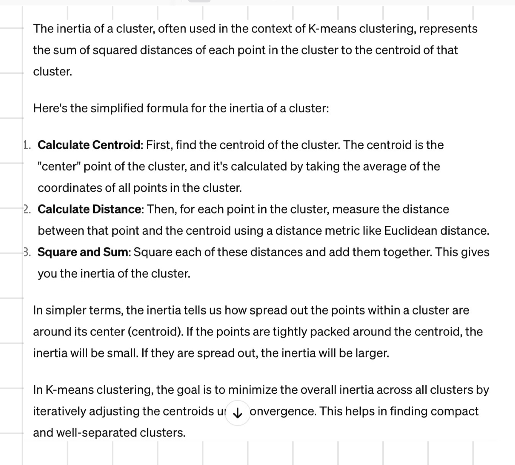
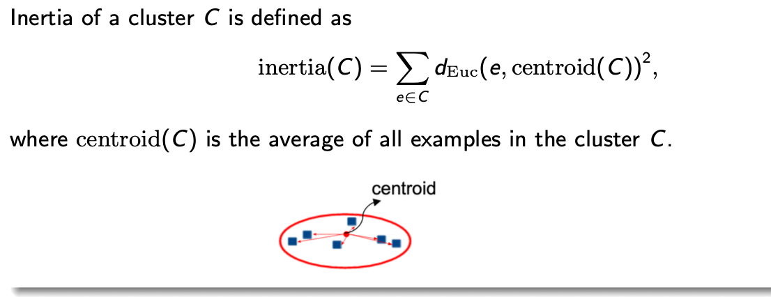
inertia of a cluster c is defined as

inertia(c) = Σe ∈ c d_euc (e, centroid(c))²

where centroid (c) is the average of all examples in the cluster c

inertia determines how compact the cluster is. Smaller the inertia, more similar the examples are within the cluster

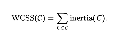
within cluster sum of squares (wcss)

of a clustering structure c consisting of k clusters is defined as

wcss(c) = Σe ∈ c inertia(c)

• the sum of the inertia of all clusters in the clustering structure

this quantifies the inertial of all clusters in the clustering structure

used to evaluate the compactness of clusters in clustering algorithms - measures total inertia/spread of all clusters in the clustering solution

optimisation problem

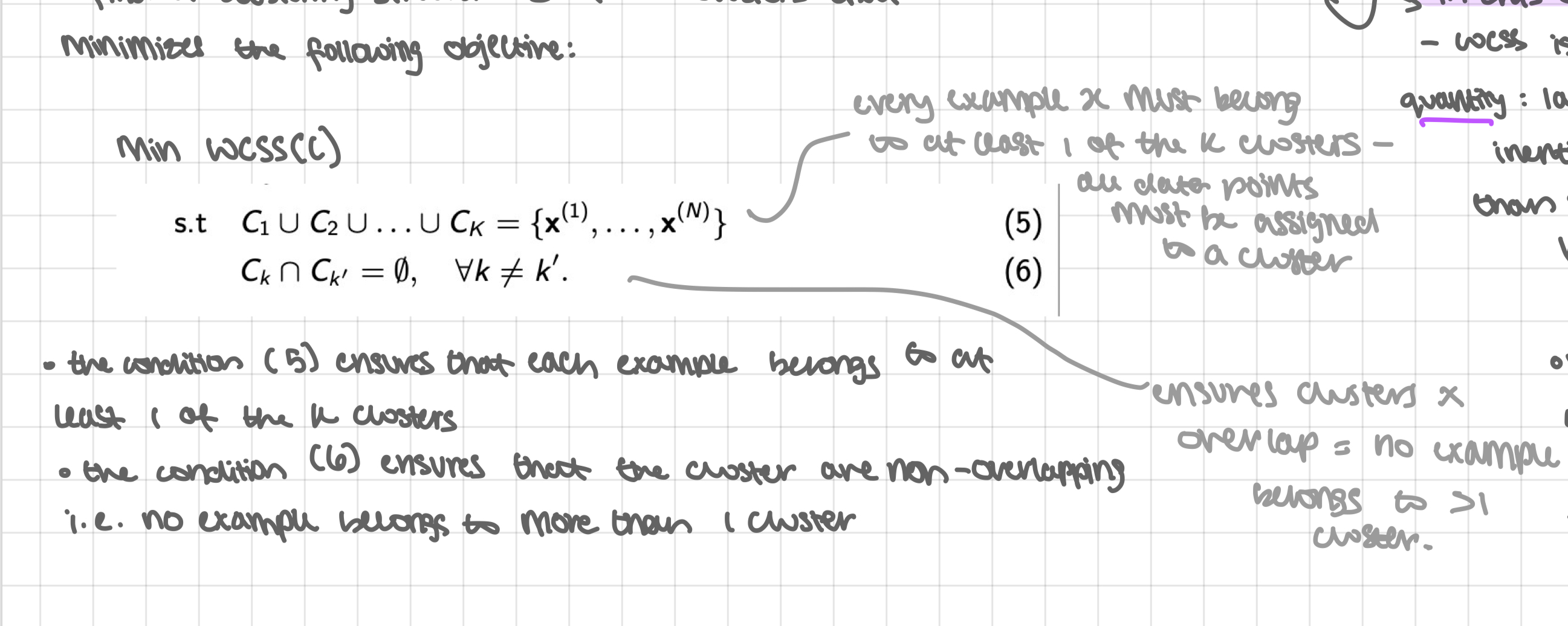
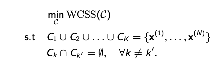
find a clustering structure c of K clusters that minimises the following objective: (see pic)

• the condition (5) ensures that each example belongs to at least 1 of the k clusters

• the condition (6) ensures that the clusters are non-overlapping i.e. no example belongs to more than 1 cluster

in this optimisation problem:

• wcss is an unnormalised quantity: larger clusters with high inertia are penalised more than smaller clusters with high inertia

• minimising wcss of a clustering structure equivalently maximises the intra-cluster similarity

solving the optimisation problem

- finding exact solution of above problem = prohibitively hard

• there are almost k^N ways to partition N observations into k clusters

• infeasible when N is large

hence → look for suboptimal approximate solutions via iterative algorithms

- includes algorithms like k-means, k-medoids

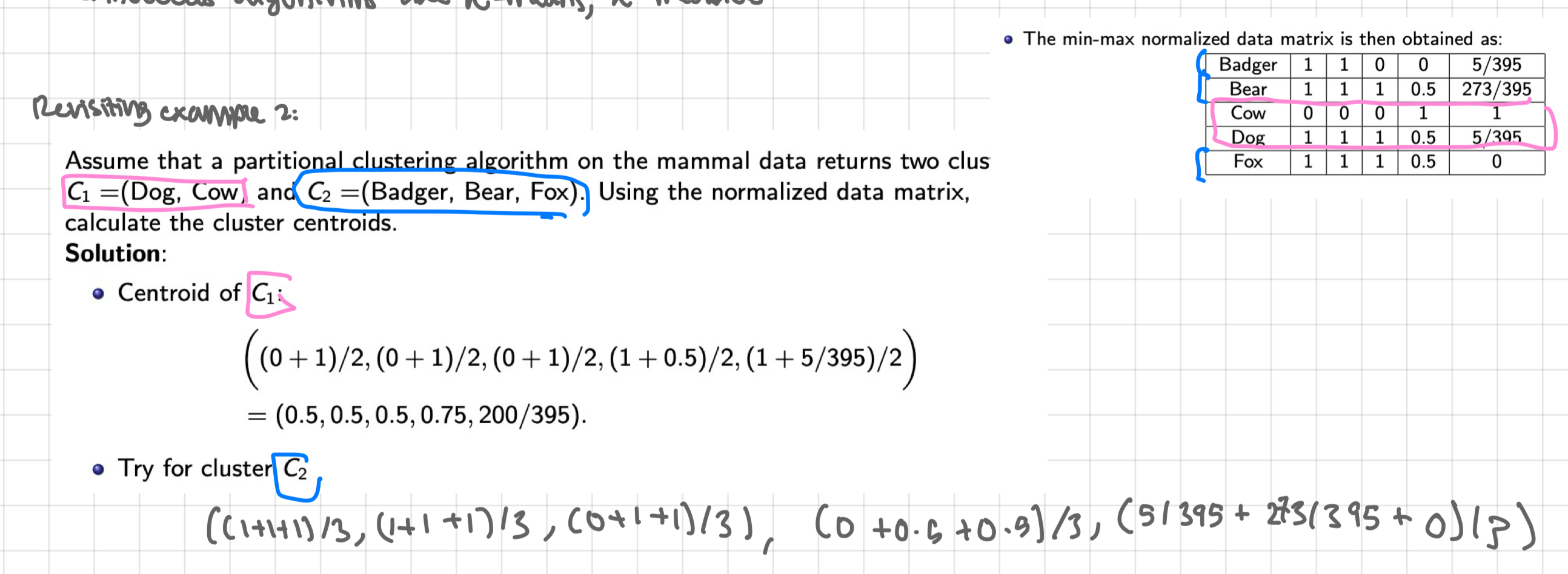
revisiting example 2

assume that a partition clustering algorithm on the mammal data returns two clusters C₁= (Dog, Cow) and C₂= (Badger, Bear, Fox). Using the normalised data matrix, calculate the cluster centroids