MA22016 Differential Equations

Define an ordinary differential equation (ODE)

An ordinary differential equation (ODE) is an equation that relates one or more state variables to their derivatives with respect to an independent variable (t, usually representing time).

Define a parameter

A parameter is a constant that appears in the ODE but does not change with respect to the independent variable. Parameters are usually denoted by the Greek letters, eg α, β and γ.

Define the order of a derivative

The order of a derivative is the number of times the differential operator is applied.

Define the order of an ODE 

The order of an ODE is the order of highest derivative.

When is an ODE autonomous?

An ODE is autonomous if it does not explicitly depend on the independent variable t.
Otherwise, it is nonautonomous.

When is an ODE homogeneous?

An ODE is homogeneous if it does not include any terms that are either constant or depend only on the independent variable.

Otherwise, it is inhomogeneous.

Describe a linear ODE

An ODE is linear if it is defined by a linear polynomial in the dependent variable and its derivatives, ie. there are no products of the independent variable with itself or any of its derivatives. 

Otherwise, it is nonlinear.

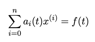
Give the general form of a linear ODE

where a(sub i)(t) and f(t) are functions of t and x^(i) is the ith derivative of x with respect to t.

Define an initial value problem (IVP)

An initial value problem (IVP) is an ODE where the value of the dependent variable is known at some prescribed value of the independent variable, usually t(sub0) = 0

Define a continuous-time dynamical system 

A continuous time dynamical system is a system composed of one or more states that evolve over time according to one or more differential equations.

Define a single first order ODE

A single first order ODE is an equation of the form xdot = f(t,x) where f is a known function of t and x that may be linear or nonlinear.

If we wish to emphasise that f also depends on the parameter μ we write xdot = f(t, x;μ)

Define a system of first order ODEs

A system of first order ODEs is a coupled set of first order ODEs. There is one equation for each state variable in the system.

If all the equations are linear, the system is a linear system. Otherwise, it is a nonlinear system.

In general, a system of n ODEs for n state variables has the form,

xdot = f (t,x)

where xdot, f and x are all vectors

x = [x1,x2,…,xn]

f = [f(sub1)(t,x), f(sub2)(t,x),…,f(subn)(t,x)]

Define the state space

The state space is the set of all possible values of the state variables.

Define the system state

The system state is the value of the state variables at a given time t.

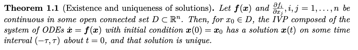
State Theorem 1.1 Existence and uniqueness of solutions

When is a problem well-posed?

A problem is said to be well-posed if,

1. a solution exists, at least over the time interval for which it is required

2. the solution is unique

3. the solution depends continuously on the initial condition and parameters

Define a steady state (or equilibrium) of an ODE

A steady state or equilibrium of an ODE is a state that does not change with time. So x* is a steady state, or equilibrium, of the ODE xdot = f(x) if f(x*) = 0.

Describe the difference between the transient part of the solution to an ODE and the asymptotic part of the solution

The transient part of the solution corresponds to the initial phase during which the initial conditions may have a strong influence on the dynamics.

The asymptotic part of the solution corresponds to the long-term behaviour after which the effect of the initial conditions has become negligible.

When is a steady state locally stable?

A steady state is locally stable if solutions that start ‘close’ to it stay ‘close’ to it. They do not move away from the steady state, but do not converge to it either.

A steady state is stable if one of the eigenvalues of the system matrix A is zero and the other, if there is one, is zero or has negative real part.

When is a steady state locally asymptotically stable?

A steady state is locally asymptotically stable if all solution trajectories that start sufficiently close to the steady state converge to it as t→∞.

Asymptotic stability corresponds to all the eigenvalues of the system matrix A being negative, or having negative real part.

When is a steady state globally asymptotically stable?

A steady state is globally asymptotically stable if all solutions that start in Ω converge to it.

When is a steady state unstable?

A steady state is unstable if all trajectories (or all but two in the case of a saddle point) that start close to the steady state move away from it as t→ ∞.

Instability corresponds to eat least one of the eigenvalues of the system matrix A being positive, or having positive real part.

Give the general form of a single first order linear ODE, and list ways to solve them

xdot + p(t)x = q(t)

• Method of undetermined coefficients

• Integrating factor method

Give the general form of a system of two linear homogeneous constant-coefficient first order ODEs.

Also give the matrix form.

x1dot = a11x1 + a12x2

x2dot = a21x1 + a22x2

where x1,x2 are state variables and aij are constants

In matrix form, xdot = Ax

where x = (x1,x2)^T and

A = (a11, a12

a21, a22)

What happens if we have a non-homogeneous linear system, xdot = Ax + b?

The non-homogeneous linear system can be transformed into a homogeneous linear system by a suitable coordinate shift.

What about second order linear differential equations? Can we convert them to linear systems?

Second order linear differential equations can be written as pairs of linear first order differential equations.

Eg. udoubledot + a1udot + a0u = b

Let x1(t) = u(t), x2(t) = udot(t). Then,

x1dot(t) = udot = x2

x2dot(t) = udoubledot = b - a1udot - a0u = b - a1x2 - a0x1

Matrix form:

x = (x1,x2)^T, b = (0,b)^T

A = ( 0 1

-a0 a1)

x = Ax + b is the corresponding linear system

Steady states are locations in state space, x*, where xdot = 0.

x does not change with time so that Ax = 0

What does it mean if A is singular, and what does it mean if A is non-singular?

If A is singular, there are infinitely many steady states.

If A is non-singular, then Ax = 0 → A^-1 A x = 0 → x = 0 is the unique solution

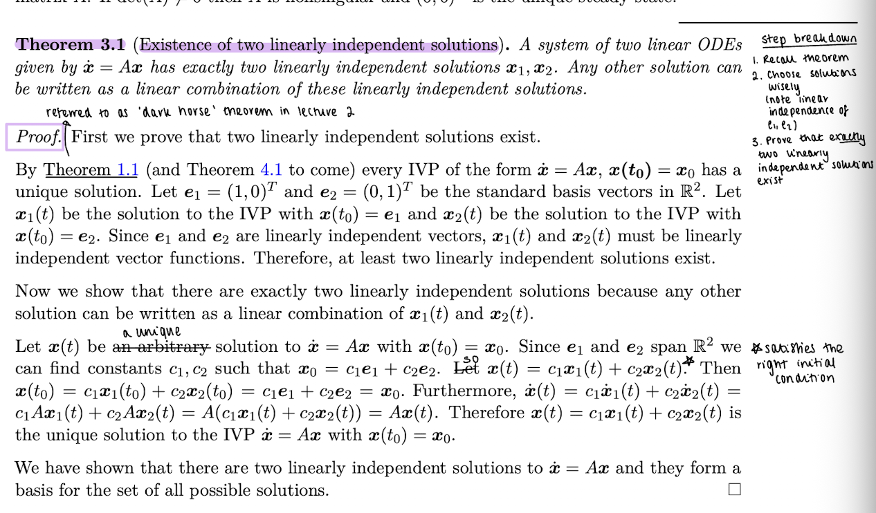
Prove theorem 3.1, that a system of two linear ODEs given by xdot = Ax has exactly two linearly independent solutions x1,x2. Any other solution can be written as a linear combination of these linearly independent solutions.

Step breakdown:

1. Recall theorem

2. Choose solutions wisely (not linear independence of e1,e2)

3. Prove that exactly two linearly independent solutions exist

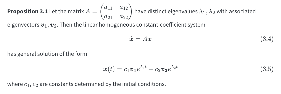
(Proposition 3.1) Let the matrix

A = (a11 a12

a21 a22)

have distinct eigenvalues λ1, λ2 with associated eigenvectors v1,v2.Then, the linear homogeneous constant-coefficient system xdot = Ax has a general solution of what form?

x(t) = c1v1e^(λ1t) + c2v2e^(λ2t)

= c1x1(t) + c2x2(t)

where c1,c2 are constants determined by the initial conditions

Prove proposition 3.1

When the eigenvalues are distinct, proposition 3.1 applies. What happens if the eigenvalues are repeated?

If λ = λ1 = λ2, and λ has two linearly independent eigenvectors v1,v2 then the general solution is,

x(t) = c1v1e^(λt) + c2v2e^(λt)

If λ = λ1 = λ2 but λ only has one linearly independent eigenvector v1, then the general solution is,

x(t) = c1v1e^(λt) + c2 (v1te^(λt) + v2e^(λt))

where v2 is a generalised eigenvector, its a solution of (A-λI)v2 = v1.

How do we classify solution structure if we have λ1,λ2 real and distinct eigenvalues with:

a) λ1<0 and λ2<0

b) λ1<0 and λ2>0

c) λ1>0 and λ2<0

d) λ1>0 and λ2>0

e) λ1=0 and λ2>0 or λ1>0 and λ2=0

f) λ1=0 and λ2<0 or λ1<0 and λ2=0

a) λ1<0 and λ2<0

• all solutions approach 0 monotonically

• x* = 0 is an asymptotically stable steady state

• a stable node

b) λ1<0 and λ2>0

• all solutions diverge from 0 except from those that start on v1, which approach 0 monotonically

• x* = 0 is an unstable steady state

• saddle, with unstable manifold v1, unstable manifold v2

c) λ1>0 and λ2<0

• x* = 0 unstable steady state

• saddle, with stable manifold v2, unstable manifold v1

d) λ1>0 and λ2>0

• all solutions diverge from 0

• x* = 0 is an unstable steady state

• an unstable node

e) λ1=0 and λ2>0 or λ1>0 and λ2=0

• x* = 0 unstable

f) λ1=0 and λ2<0 or λ1<0 and λ2=0

• x* = 0 stable, but not asymptotically stable

• solutions do not diverge from 0 but do not approach it either

What is the general solution if the eigenvalues are a complex conjugate pair, λ = a +- bi, b≠0?

x(t) = c1ve^(λt) + c2v~e^(λ~t) where λ, λ~, v, v~ are complex conjugate pairs.

In general, x(t) is complex-valued

Construct a real-valued solution from the complex-valued solution

From the complex-valued solution, we can construct a real-valued solution:

x(t) = e^(at) (u1cos(bt) + u2sin(bt))

are not eigenvectors of A, rather they are derived from the eigenvectors.

Interpret the components of the real-valued solution:

x(t) = e^(at) (u1cos(bt) + u2sin(bt))

The sine and cosine terms give rise to oscillations in the solution trajectories with period determined by imaginary part of the eigenvalues.

The real part of the eigenvalues determines whether trajectories get closer to the origin, move away from it, or remain at a fixed distance.

In the phase plane, trajectories appear as spirals or closed loops.

If Re(λ) < 0, the steady state is asymptotically stable. It is called a stable focus or spiral sink. Solution trajectories in the phase plane spiral into the steady state.

If Re(λ) > 0, the steady state is unstable. It is called an unstable focus or spiral source. Solution trajectories in the phase plane spiral out from the steady state.

If Re(λ) = 0, solution trajectories oscillate with fixed amplitude around the steady state, forming closed loops in the phase plane. The steady state is a centre which is stable, but not asymptotically stable. This is sometimes termed neutrally stable.

What are the Routh-Hurwitz criteria for?

The Routh-Hurwitz criteria provide a simple way to determine the stability of a steady state without having to calculate the eigenvalues.

What are the Routh-Hurwitz criteria?

The criteria state that for a system of two linear equations, the eigenvalues of the system matrix A all have negative real part, and x* = 0 is an asymptotically stable steady state, if and only if,

β = trA < 0

and γ = det A > 0

Prove Lemma 4,1, that is that for any n∈N, any linear ODE (or IVP) of order n can be written as a system of n linear first order ODEs (or IVPs)

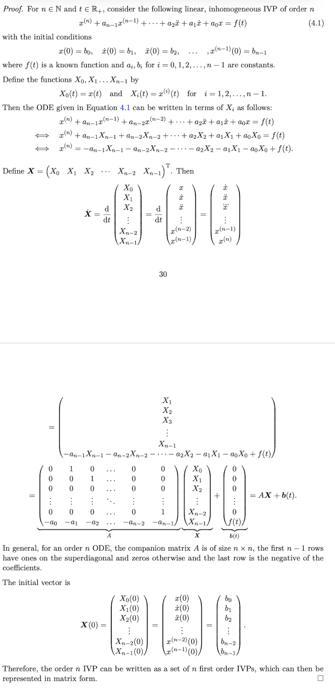
When converting a single n-th order ODE for x(t) into a system of first-order ODEs, how is the vector function X(t) defined?

X(t) = (x xdot xdoubledot …. x(n-1) )^T

The vector consists of the dependent variable and its derivatives up to the (n-1)th order.

If a function x(t) is a solution to an n-th order linear ODE, how does it relate to the corresponding linear system Xdot = AX + f?

The vector function X(t) (constructed from x(t) and its derivatives) is a solution to the system Xdot = AX + f

If a vector function X(t) is a solution to the system Xdot = AX + f (derived from an n-th order ODE), which component provides the solution to the original higher-order ODE?

The first component of the vector X(t) is the solution to the original n-th order ODE.

What about coupled higher order ODEs?

Coupled higher order ODEs can be converted into a system of first order ODEs using the same process as for a single higher order equation.

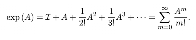
Define the matrix exponential function

Let n∈N, I be the nxn identity matrix and A be an nxn matrix.

The matrix exponential function (MEF) of A is denoted exp(A) and defined as,

(see image)

O is the nxn zero matrix.

exp(O) =

I (nxn identity matrix)

exp(A) exp(-A) =

I

exp(A^T) =

exp(A)^T

Let A* denote the conjugate transpose of A.

exp(A*) =

exp(A)*

If A and B are commutative (ie AB = BA), then exp(A)exp(B) =

exp(A + B)

If A is invertible, exp(ABA^(-1)) =

A exp(B) A^(-1)

For λ, μ are constants, exp(λA) exp(μA) =

exp((λ+μ)A)

What is exp(At)?

exp(At) is an infinite polynomial, which converges for all t ∈ R+.

For fixed t0 ∈ R, Aexp(A(t-t0)) =

exp(A(t-t0)) A

If A is a diagonal matrix, what form does exp(A) take?

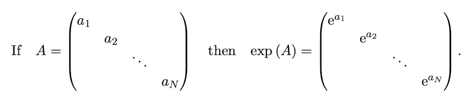
What is the derivative of exp(A(t-t0)) with respect to t?

d/dt exp(A(t-t0)) = Aexp(A(t-t0)) = exp(A(t-t0)) A

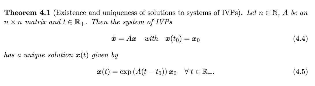
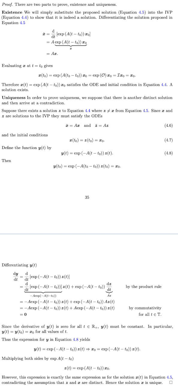
State Theorem 4.1 (Existence and uniqueness of solutions to systems of IVPs)

Let n∈N, A be an nxn matrix and t∈R+. Then, the system of IVPs,

xdot = Ax with x(t0) = x0

has a unique solution x(t) given by

x(t) = exp(A(t-t0))x0 for all t∈R+

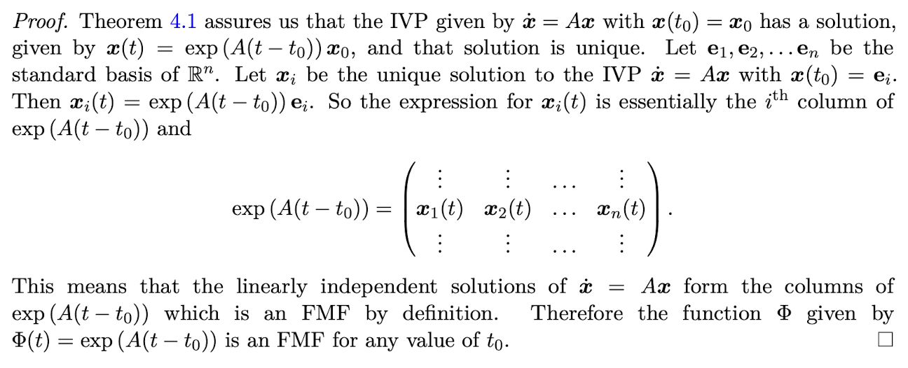
Prove Theorem 4.1

According to Theorem 4.2, how many linearly independent solutions does the system xdot = Ax (where A is an nxn matrix) have, and how is the general solution expressed?

The system has exactly n linearly independent solutions (x1, x2, .., xn)

Any arbitrary solution x(t) is a linear combination of these solutions:

x(t) = (sum from i=1 to n) ci xi(t) where ci are constants determined by initial conditions

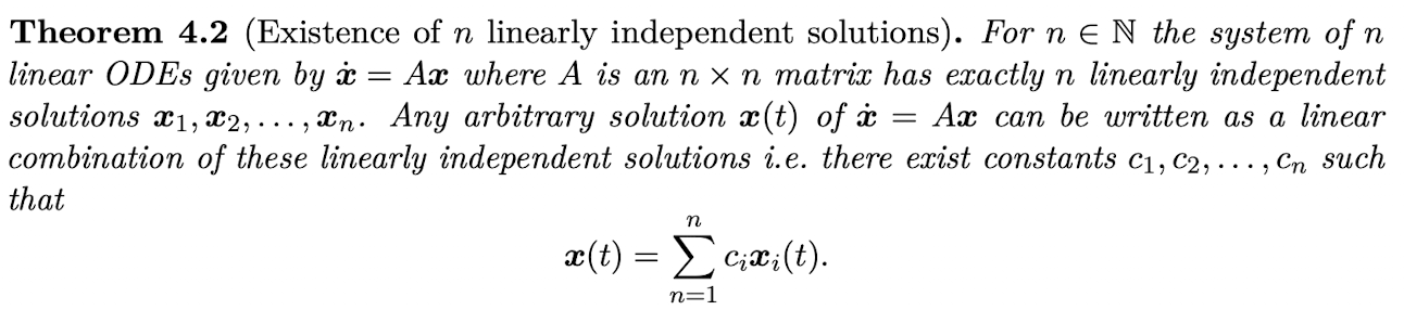
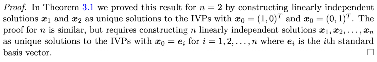
Prove Theorem 4.2

Define an eigenpair

For an nxn matrix A, the eigenvalue λ and corresponding eigenvector v, can be represented as an eigenpair {λ, (v)}

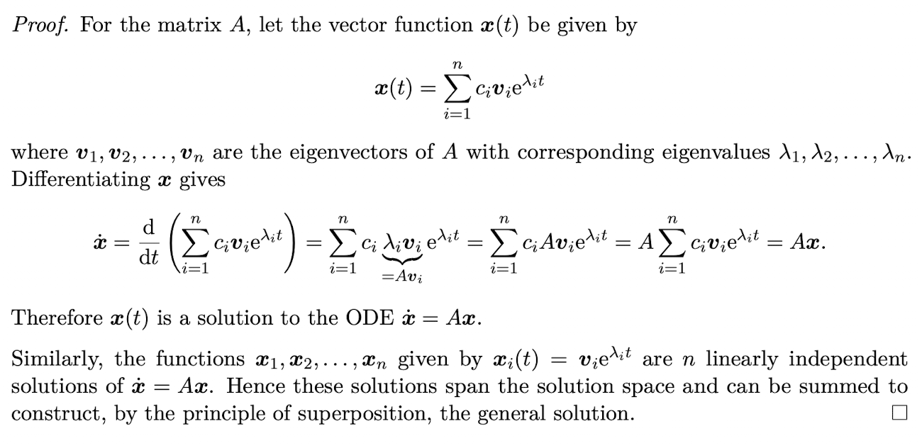
(Theorem 4.3) Let n∈N and A be an nxn matrix with n linearly independent eigenvectors v1, v2,…,vn corresponding to the n eigenvalues λ1, λ2,..,λn. Then, what is the general solution to the ODE xdot = Ax?

x(t) = (sum from i=1 to n) ci vi e^(λit) for some constants c1,c2,…,cn

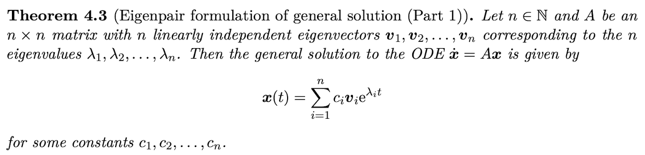
Prove Theorem 4.3

Define a generalised eigenvector

Let A be an nxn matrix, and λ be an eigenvalue of A. Then, a vector v is a generalised eigenvector of order k corresponding to λ if,

(A - λI)^k v = 0 but (A - λI)^i v ≠ 0 for all i = 1,2,…,k-1

Let A be an nxn matrix. How mnay linearly independent generalised eigenvectors must A have?

A must have n linearly independent generalised eigenvectors.

What is the order of a standard eigenvector?

A standard eigenvector is a generalised eigenvector of order 1.

Define a characteristic polynomial

Let A be an nxn matrix. The characteristic polynomial, or characteristic equation of A is the polynomial in λ of degree n given by

P(λ) = | A - λI |

Define algebraic multiplicity

The algebraic multiplicity ma(λ) of an eigenvalue λ of A is the number of times it appears as a root of the characteristic polynomial P(λ).

Define geometric multiplicity

The geometric multiplicity mg(λ) of an eigenvalue λ of A is the number of linearly independent eigenvectors corresponding to λ, ie. the dimension of the subspace spanned by the eigenvectors of λ.

Give the inequality showing the relationship between algebraic and geometric multiplicities

1 <= mg(λ) <= ma(λ)

How do we find the number of generalised eigenvectors of order 2 or greater, given algebraic and geometric multiplicity?

Number of generalised eigenvectors (of order 2 or greater) = ma(λ) - mg(λ)

(Theorem 4.4) For a repeated eigenvalue λ with eigenvector v1 and generalised eigenvector v2, what is the second linearly independent solution x2(t)?

x2(t) = e^(λt) (v2 + v1t)

(notice that t is attached to the standard eigenvector)

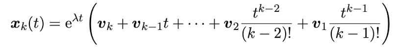
(Theorem 4.4) What is the formula for the k-th solution xk(t) involving a chain of generalised eigenvectors?

(see image)

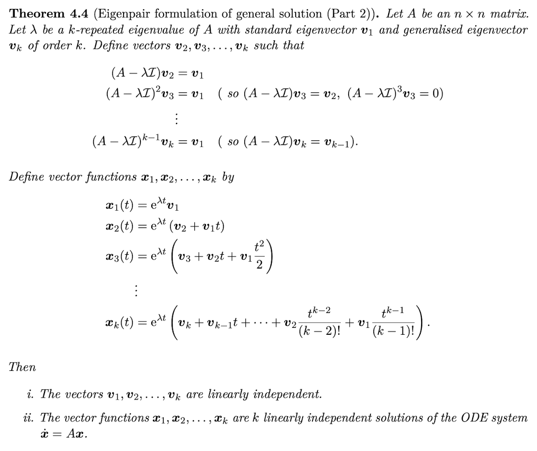
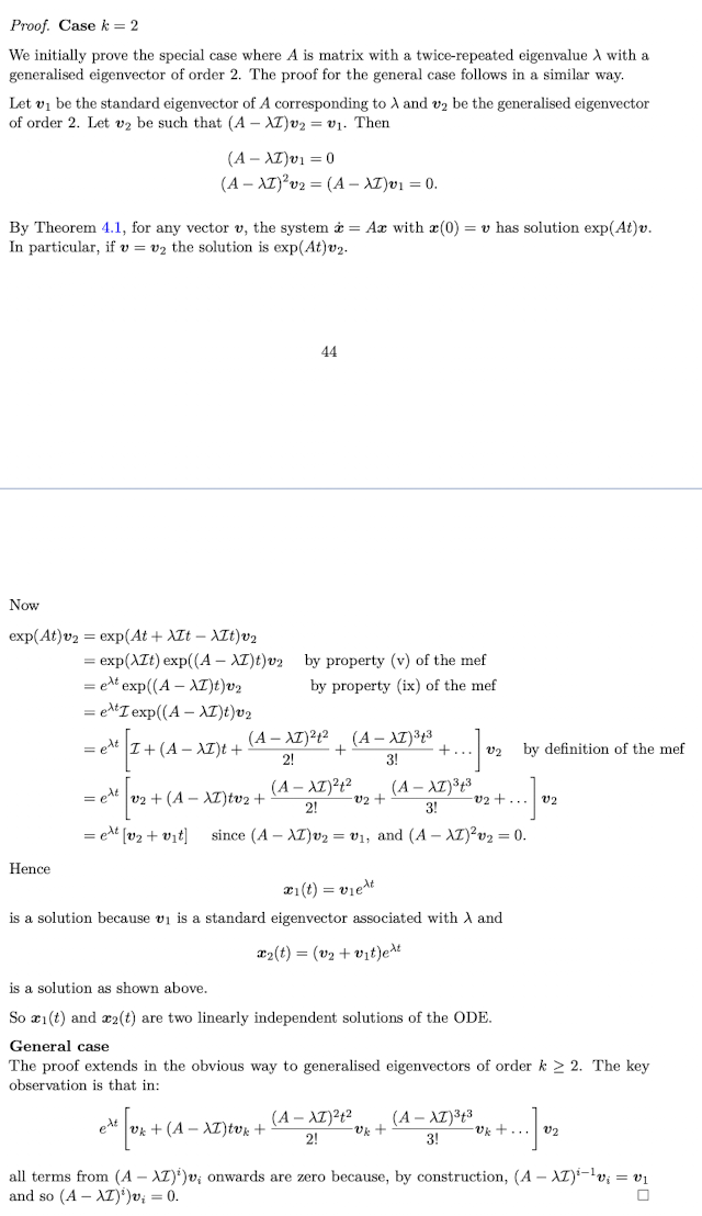
Prove Theorem 4.4

Define a fundamental matrix function (FMF)

Let A be an nxn matrix. A fundamental matrix function (FMF) associated with the system of n linear homogeneous constant-coefficient differential equations xdot = Ax is a matrix valued function Φ(t) such that the columns of Φ are linearly independent solutions of the ODE.

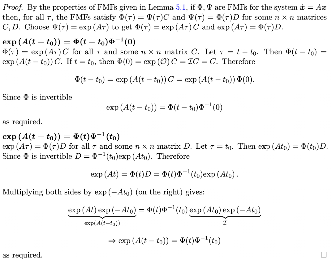
Prove that the matrix exponential function is a fundamental matrix function. That is, that for an nxn matrix A, the function Φ given by Φ(t) = exp(A(t-t0)) is an FMF of xdot = Ax for any value of t0.

(Lemma 5.1) Let A be an nxn matrix. Let φ and ψ be two FMFs for A. Then for any t0, and all t>t0, prove that:

• There exists an nxn matrix C such that φ(t) = ψ(t)C

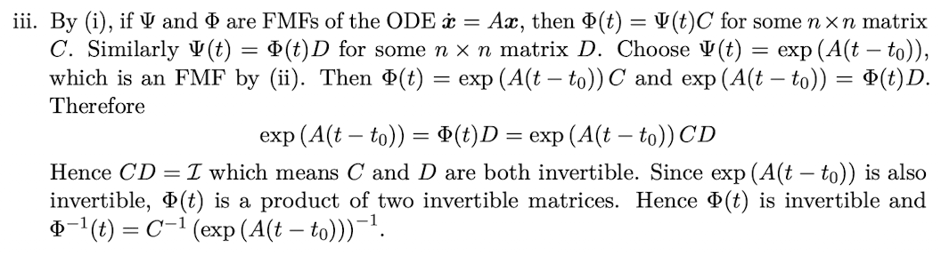
(Lemma 5.1) Let A be an nxn matrix. Let φ and ψ be two FMFs for A. Then for any t0, and all t>t0, prove that:

• The matrix φ(t) can be written as φ(t) = exp(A(t-t0))C for some nxn matrix C

(Lemma 5.1) Let A be an nxn matrix. Let φ and ψ be two FMFs for A. Then for any t0, and all t>t0, prove that:

• The matrix φ(t) is invertible

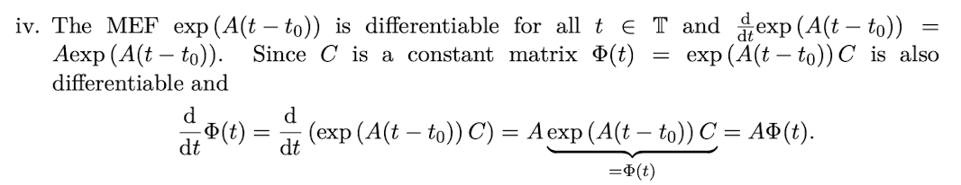
(Lemma 5.1) Let A be an nxn matrix. Let φ and ψ be two FMFs for A. Then for any t0, and all t>t0, prove that:

• The matrix φ(t) is differentiable (component-wise) with derivative d/dt φ(t) = Aφ(t)

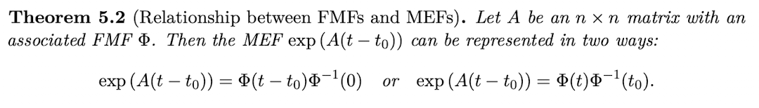
(Theorem 5.2) Let A be an nxn matrix with an associated FMF φ. Then how can the MEF exp(A(t-t0)) be expressed? (Two ways)

exp(A(t-t0)) = φ(t-t0) φ^(-1)(0)

exp(A(t-t0)) = φ(t) φ^(-1)(t0)

Prove Theorem 5.2

(Theorem 5.3) Let A be an nxn matrix. What is the unique solution x(t) to the IVP xdot = Ax with x(t0) = x0 written in terms of an FMF φ?

x(t) = φ(t-t0) φ^(-1)(0) x0 or x(t) = φ(t) φ^(-1)(t0) x0
note that the first form is useful because it does not require computing an infinite series of powers of A

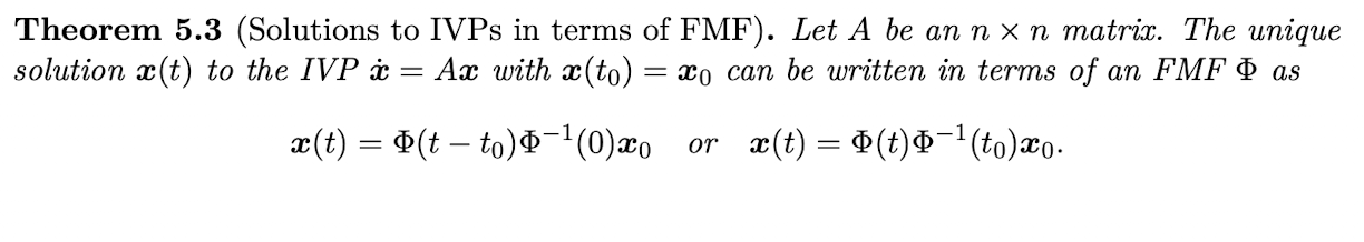
Prove Theorem 5.3

Define an asymptotically stable system of linear ODEs

A system of linear ODEs xdot = Ax is asymptotically stable if every solution x(t) → 0 as t → ∞

Define an asymptotically stable steady state of a system of linear ODEs

The steady state 0 of the system of linear ODEs xdot = Ax is asymptotically stable if every solution x(t) → 0 as t → ∞

Define an asymptotically stable matrix

An nxn matrix A is asymptotically stable if every eigenvalue of A has negative real part.

Define an asymptotically stable polynomial

A polynomial is asymptotically stable if every root has negative real part

State Proposition 6.1, Equivalence of stability definitions

Let A be an nxn matrix with characteristic polynomial P(λ). Then, A is stable if and only if P(λ) is stable, if and only xdot = Ax is stable, if and only if 0 is an asymptotically stable steady state of xdot = Ax.

Note the difference between the stability of an ODE and an IVP (Remark 6.2)

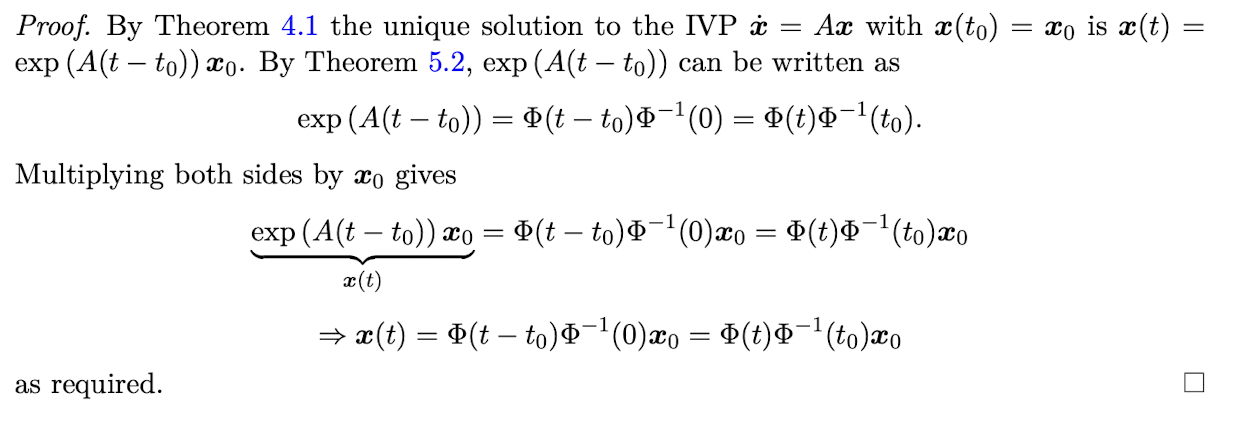
Define the Hurwitz matrices

State Theorem 6.1, Routh-Hurwitz stability criteria

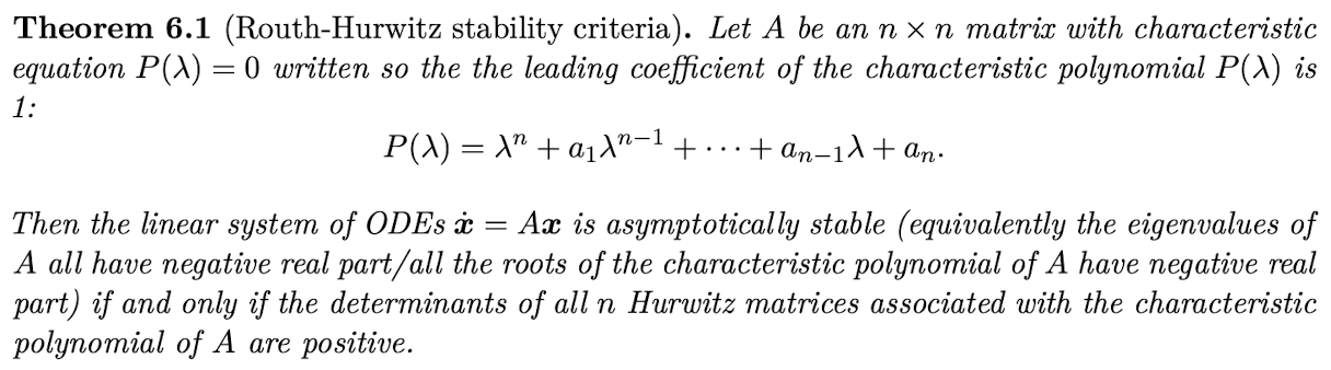
State the Routh-Hurtwitz criterion for n=2

Let A be a 2×2 matrix with characteristic equation λ² + a1λ + a2 = 0. Then, the system of ODEs xdot = Ax is asymptotically stable if and only if a1>0 and a2>0. Note that a1 = -tr(A), a2 = det(A).

State the Routh-Hurwitz criterion for n=3

Let A be a 3×3 matrix with characteristic equation λ³ + a1λ² + a2λ + a3 = 0. Then the system of ODEs xdot = Ax is asymptotically stable if any only if a1>0, a3>0 and a1a2>a3.

What is the general form of the single first order nonlinear ODEs considered in this course?

xdot = f(t,x)

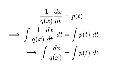
REVIEW Define a separable equation

A first-order ordinary differential equation is separable if it can be written in the form dx/dt = p(t)q(x)

We can solve separable equations directly by integration, as shown in the image.

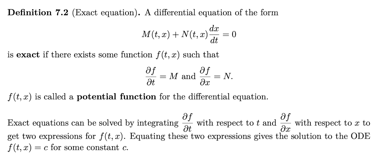
REVIEW Define an exact equation

See image

REVIEW Define a Bernoulli differential equation

See image

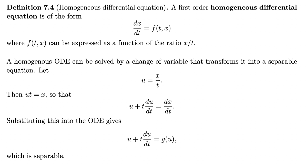
REVIEW Define a homogeneous differential equation

See image

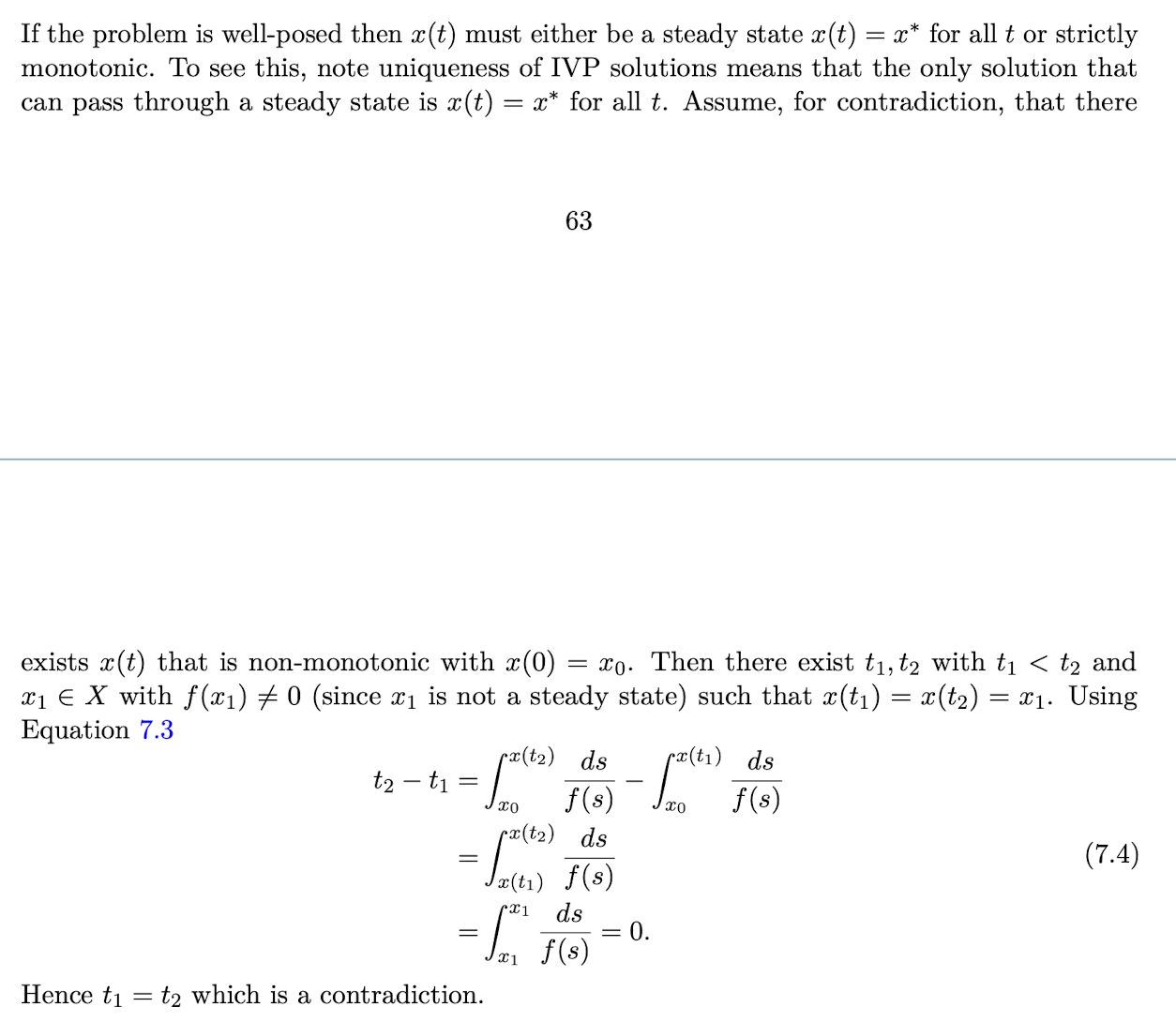
Show the uniqueness of IVP solutions for first order autonomous ODEs

Why do we use phase-line diagrams?

Phase-line diagrams can be used to explore the qualitative properties of a first order autonomous ODE without finding its analytical solution.

They are easy to sketch, and can offer quick insights into solution behaviour.

Give the steps for constructing a phase-line diagram for the ODE xdot = f(x)

1. Plot f(x) as a function of x

2. Mark points where f(x) crosses the x-axis as steady states

3. In regions where f(x)>0, xdot>0 so x(t) is increasing with t. Draw an arrow on the x-axis pointing in the direction of increasing x

4. In regions where f(x)<0, xdot<0 so x(t) is decreasing with t. Draw an arrow on the x-axis pointing in the direction of decreasing x.

What is linear stability analysis useful for?

Linear stability analysis is used to determine whether the steady state of a nonlinear equation is locally stable or unstable. It can also tell us how quickly the solution approaches or moves away from a steady state if it starts close to it.