Gradients, Slice Selection, Frequency Encoding (9.1 - 9.3)

NOTE

Read the note explaining Gradients

What is the role of gradient coils in MRI?

Gradient coils in MRI are used to vary the strength of the main magnetic field ($B_0$) along different axes (x, y, z). This variation allows the system to spatially encode the location of protons by adjusting their resonant (Larmor) frequencies.

How are gradient coils mathematically represented?

The gradient field is represented as:

$B = \left(B_0 + G_x x + G_y y + G_z z \right) \hat{z} = (B_0 + \mathbf{G} \cdot \mathbf{r}) \hat{z}$

Here:

- $B_0$: Main magnetic field strength.

- $G_x, G_y, G_z$: Gradient strengths along the x, y, and z directions.

- $\mathbf{r} = (x, y, z)$: Position vector.

- $\mathbf{G} = (G_x, G_y, G_z)$: Gradient vector.

What is the significance of gradient coil switching?

Switching gradient coils on and off rapidly (0.1–1 ms) enables precise control of magnetic field variation and spatial encoding of signals. This rapid switching, called the slew rate, is typically 5–250 mT m$^{-1}$ s$^{-1}$ and must be carefully managed to avoid inducing eddy currents in the patient.

How do gradients contribute to MRI image formation?

Gradients allow selective excitation of protons at specific spatial locations by modifying their resonant frequencies. The spatial information is encoded in the signal phase and frequency, enabling reconstruction of the image through the Larmor frequency and transverse magnetization phase.

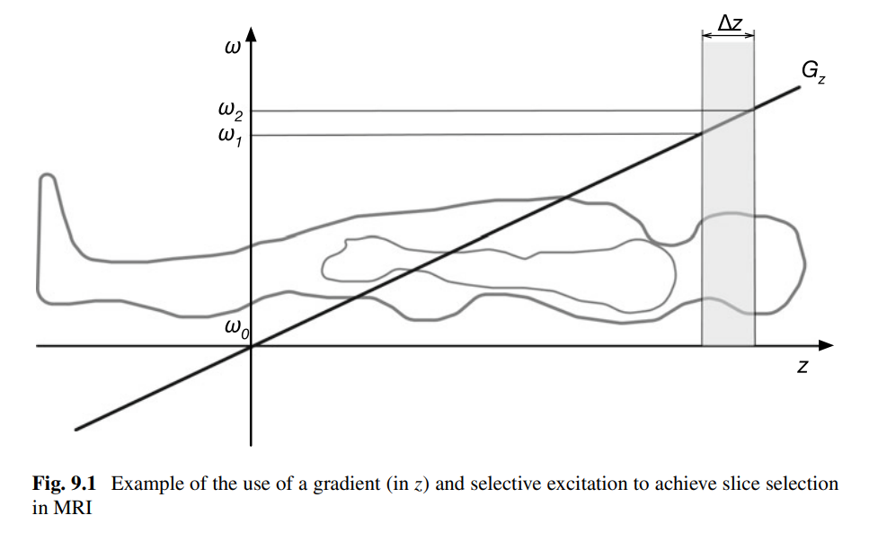
What is the purpose of slice selection in MRI?

Slice selection ensures that the received signal only comes from a specific slice of tissue. This is achieved by applying a gradient $G = (G_x, G_y, G_z)$, which creates a Larmor frequency variation depending on the spatial location.

What happens to the Larmor frequency with a gradient?

The Larmor frequency becomes position-dependent:

$\omega(r) = \gamma(B_0 + G \cdot r)$

If we want to select a specific slice at $z$, we apply a gradient $G = (0, 0, G_z)$, making the Larmor frequency:

$\omega(z) = \gamma(B_0 + G_z z)$

Why can’t we excite an infinitesimally thin slice in practice?

- RF pulses have finite bandwidth, so a precise sinusoidal waveform cannot be delivered.

- Signals depend on the number of protons in the slice, and a very thin slice would not provide enough signal for detection.

How is slice selection achieved in practice?

A range of RF frequencies is applied to excite a thick slice or slab over the frequency range $[ \nu_1, \nu_2 ]$. The slice thickness depends on the combination of:

- RF frequency range (bandwidth $\Delta \omega = \omega_2 - \omega_1$)

- Gradient strength ($G_z$)

- RF center frequency ($\bar{\omega} = (\omega_1 + \omega_2)/2$)

What are the three parameters for controlling slice position and thickness?

1. $G_z$: z-gradient strength.

2. $\bar{\omega}$: RF center frequency.

3. $\Delta \omega$: RF frequency range (bandwidth).

What is the relationship between slice thickness and slice position, and how can you calculate RF bandwidth for slice selection?

Fundamental Equations:

1. Larmor Frequency: $\omega = \gamma (B_0 + G_z z)$

2. Slice Position: $z_1 = \frac{\omega_1 - \gamma B_0}{\gamma G_z}$, $z_2 = \frac{\omega_2 - \gamma B_0}{\gamma G_z}$

3. Mean Slice Position: $\bar{z} = \frac{\bar{\omega} - \omega_0}{\gamma G_z}$

4. Slice Thickness: $\Delta z = \frac{\Delta \omega}{\gamma G_z}$

5. RF Bandwidth: $\Delta \nu = \gamma G_z \Delta z$

Steps for Derivation of Slice Thickness and Position:

1. Relationship for Slice Position (Mean, $\bar{z}$):

- Slice position is determined using the center frequency $\bar{\omega}$. The gradient strength $G_z$ and gyromagnetic ratio $\gamma$ relate it to the $z$-position:

$z_1 = \frac{\omega_1 - \gamma B_0}{\gamma G_z}, \quad z_2 = \frac{\omega_2 - \gamma B_0}{\gamma G_z}$

- Mean position $\bar{z}$ is calculated as the average of $z_1$ and $z_2$:

$\bar{z} = \frac{z_1 + z_2}{2} = \frac{1}{\gamma G_z}\left(\frac{\omega_1 + \omega_2}{2} - \gamma B_0 \right)$

or:

$\bar{z} = \frac{\bar{\omega} - \omega_0}{\gamma G_z}$

2. Relationship for Slice Thickness ($\Delta z$):

- Slice thickness is the difference between $z_2$ and $z_1$:

$\Delta z = z_2 - z_1 = \frac{\omega_2 - \omega_1}{\gamma G_z}$

or:

$\Delta z = \frac{\Delta \omega}{\gamma G_z}$

3. Calculate RF Bandwidth ($\Delta \nu$):

- Using the equation for $\Delta z$, solve for RF bandwidth $\Delta \nu$:

$\Delta \nu = \gamma G_z \Delta z$

- Substitute values:

$\gamma = 42.58 \times 10^6 \, \text{Hz/T}, \, G_z = 40 \, \text{mT/m}, \, \Delta z = 5 \, \text{mm} = 5 \times 10^{-3} \, \text{m}$

$\Delta \nu = 42.58 \times 10^6 \times 40 \times 10^{-3} \times 5 \times 10^{-3} = 8.5 \, \text{kHz}$

What is the trade-off in slice selection for imaging a volume?

A thicker slice results in higher signal-to-noise ratio (SNR) but poorer resolution in the slice direction. Conversely, thinner slices give better resolution but may reduce SNR and contrast-to-noise ratio (CNR).

What are the consequences of slice selection depending on RF pulses?

RF pulses with a specific range of frequencies are required to define slices. Perfectly defined slice edges are not achievable because RF pulses cannot perfectly deliver only the desired frequencies, leading to extra components due to the pulse shape and duration.

Why are small gaps left between slices in multi-slice MRI?

Small gaps help reduce overlap or interference between adjacent slices, improving the overall quality of the MRI. Optimizing RF pulse shape is also critical for high-quality images.

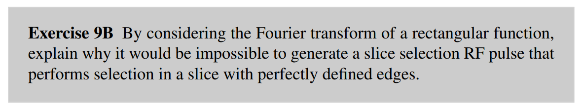
The Fourier transform of a rectangular function is a sinc function. To get a perfect slice selection we need a pulse that only has frequencies in a specific range, i.e. the bandwidth, and equal magnitude at all frequencies within the bandwidth. Thus, the pulse needs to generate a rectangular function in the frequency domain, this would require a sinc pulse in the time-domain. However, a sinc function has many side lobes and thus cannot be generated in a finite duration pulse. In reality careful shaping of the RF pulse will be required to get as precise a slice selection as possible.

What is the equation for transverse magnetization after a pulse?

$M_{xy}(t) = M_{xy}(0^+) e^{-j(2\pi \omega_0 t - \phi)} e^{-t/T_2}$ (Eq. 9.4)

Magnetisation in the horizontal plane when protons are tilted.

What is $M_{xy}(0^+)$?

$M_{xy}(0^+) = M_z(0^-) \sin \alpha$, where $M_z(0^-)$ is the longitudinal magnetization before the pulse and $\alpha$ is the flip angle. (Eq. 9.5)

What is the received signal in MRI?

$s(t) = \iint A M_{xy}(x, y, 0^+) e^{-j2\pi \omega_0 t} e^{-t/T_2(x, y)} dx dy$, where:

- $A$: Scanner-specific gain,

- $M_{xy}(x, y, 0^+)$: Transverse magnetization immediately after excitation,

- $\omega_0$: Larmor frequency,

- $T_2(x, y)$: Spin-spin relaxation time. (Eq. 9.6)

What assumption is made for simplicity in Eq. 9.6?

The phase $\phi$ is assumed to be zero, and the spatial variation of $M_{xy}$ and $T_2$ is explicitly noted.

What is the equation for the received signal in terms of the effective spin density, and how is it derived?

The received signal integrates over the transverse magnetization within the slice and is given as:

$s(t) = e^{-j2\pi \omega_0 t} \iint_{-\infty}^{\infty} f(x, y) \, dx \, dy$

Here, $f(x, y)$, the effective spin density, combines all the relevant parameters of the tissue and the scanner:

$f(x, y) = A M_{xy}(x, y, 0^+) e^{-t/T_2(x, y)}$

- $A$: Scanner-specific gain, related to the receive electronics.

- $M_{xy}(x, y, 0^+)$: Transverse magnetization immediately after excitation.

- $e^{-t/T_2(x, y)}$: Decay of the transverse magnetization due to $T_2$ relaxation over time.

This signal reflects the sum of contributions from all protons within the selected slice.

What is demodulation, and why is it used in MRI?

Demodulation is the process of removing the high-frequency carrier signal (oscillating at the Larmor frequency) from the received MRI signal to extract the meaningful low-frequency components.

- In MRI, the received signal is modulated at the Larmor frequency $\omega_0$.

- Demodulation shifts the signal to the "baseband," where it represents the actual spatial information.

What is the baseband signal?

The baseband signal is the low-frequency component of the MRI signal after demodulation, containing all the spatial information about the tissue being imaged.

- It simplifies the representation of the received signal for further processing.

- In the equation $s_0(t) = e^{j2\pi \omega_0 t}s(t)$, demodulation removes $e^{-j2\pi \omega_0 t}$, leaving only the spatially dependent signal.

What is the demodulated signal (baseband) we receive, and why is it necessary?

$s(t) = e^{-j2\pi \omega_0 t} \iint_{-\infty}^{\infty} f(x, y) \, dx \, dy$

The demodulated signal removes the carrier frequency $\omega_0$ to simplify further processing. It is written as:

$s_0(t) = e^{+j2\pi \omega_0 t} s(t) = \iint_{-\infty}^{\infty} f(x, y) \, dx \, dy$

- This step removes the oscillations due to $e^{-j2\pi \omega_0 t}$, leaving only the integral over the effective spin density.

- However, this step also eliminates all spatial information, as the dependency on $x$ and $y$ is lost.

- To recover spatial details, we need spatial encoding through gradients.

Why do we need a readout gradient, and what does it do?

A readout gradient is applied to encode spatial information along a specific axis (e.g., x-axis). This gradient causes the Larmor frequency to vary with the position along that axis:

$\omega(x) = \gamma (B_0 + G_x x) = \omega_0 + \gamma G_x x$

- $G_x$: Strength of the gradient in the x-direction.

- $\omega_0$: The base Larmor frequency without gradients.

The varying frequency ensures that spins at different positions along the x-axis precess at different rates, allowing their spatial location to be encoded into the signal.

How does the received signal change with a readout gradient?

The signal becomes spatially dependent on $x$, while still integrating over $y$:

$s(t) = \iint_{-\infty}^{\infty} A M_{xy}(x, y, 0^+) e^{-j2\pi (\omega_0 + \gamma G_x x)t} e^{-t/T_2(x, y)} \, dx \, dy$

Breaking this down:

- $A M_{xy}(x, y, 0^+)$: The initial transverse magnetization of the spins within the tissue.

- $e^{-j2\pi \omega_0 t}$: The base oscillation due to the main field $B_0$.

- $e^{-j2\pi \gamma G_x x t}$: The additional phase due to the gradient $G_x$, which encodes the spatial location along the x-axis.

- $e^{-t/T_2(x, y)}$: The decay of the transverse magnetization due to $T_2$ relaxation.

What is the final simplified form of the signal with spatial encoding?

Using the spatially dependent Larmor frequency $\omega(x) = \omega_0 + \gamma G_x x$, the signal simplifies to:

$s(t) = e^{-j2\pi \omega_0 t} \iint_{-\infty}^{\infty} A M_{xy}(x, y, 0^+) e^{-j2\pi \gamma G_x x t} e^{-t/T_2(x, y)} \, dx \, dy$

This equation incorporates spatial encoding along $x$, enabling the reconstruction of spatially dependent information in the final image.

What is the baseband signal obtained using the readout gradient?

Old without gradient: $s_0(t) = e^{+j2\pi \omega_0 t} s(t) = \iint_{-\infty}^{\infty} f(x, y) \, dx \, dy$

The baseband signal after demodulation is given by:

$s_0(t) = \iint_{-\infty}^{\infty} f(x, y) e^{-j2\pi \gamma G_x t x} \, dx \, dy$

This represents the integral over the effective spin density $f(x, y)$ with spatial encoding along the x-axis due to the readout gradient $G_x$.

$F(u, v) = \int_{-\infty}^{\infty} \int_{-\infty}^{\infty} f(x, y) e^{-2\pi i (ux + vy)} , dx , dy$

How does the baseband signal relate to a 2D Fourier Transform?

$F(u, v) = \int_{-\infty}^{\infty} \int_{-\infty}^{\infty} f(x, y) e^{-2\pi i (ux + vy)} , dx , dy$

$s_0(t) = \iint_{-\infty}^{\infty} f(x, y) e^{-2\pi i(\gamma G_x t x)} \, dx \, dy$

The baseband signal is equivalent to a 2D Fourier transform of the spin density $f(x, y)$, where:

- Spatial frequency in the x-direction: $u = \gamma G_x t$

- Spatial frequency in the y-direction: $v = 0$

What is k-space, and how is it represented in MRI?

In MRI, the Fourier space where spatial frequencies are sampled is called k-space.

- $k_x = u = \gamma G_x t$: Wave number in the x-direction.

- $k_y = v = 0$: Wave number in the y-direction.

The concept of k-space simplifies the representation of spatial frequency data collected during the scan.

---

2D Fourier plot starts from origin (0,0)

Horizontal Axis (u-axis): Represents the horizontal spatial frequency.  

• Higher values on this axis correspond to faster variations in the horizontal direction of the original image or signal.

Vertical Axis (v-axis): Represents the vertical spatial frequency.  

• Higher values on this axis correspond to faster variations in the vertical direction of the original image or signal.

• This means there is no vertical variation in frequency for the k-plane.