Quantity Theory of Money: The Theory to Explain Money's Long-Run Effects

What is the quantity theory of money?

In an economy with flexible prices, output and other real variables are at their long-run equilibrium. Changes in money will influence the general price level. The QUANTITY THEORY OF MONEY is a theoretical device for modelling this idea.

MV = PT where M is money in circulation, V is the (Transactions) velocity of circulation, P is the general price level, T is the volume of transactions.

The monetary value of transaction being undertaken (PT) in a given period of time must be equal to the flow of money to make those transactions happen (MV) during the dame time period.

We need to introduce output rather than use transactions. We do this by associating the production and sale of output during a period of time with a volume of transactions.

Quantity theory with OUTPUT

MV = PY, where Y is level of output and V is the income velocity of money.

We assume long-run equilibrium, so Y=Y*, also imposing constant V=V*. We get:

M= λP where λ=Y*/V*

There is a PROPORTIONAL relationship between general level of prices and money supply.

Velocity (V) is constant as over long periods of time we would expect transaction technology to change, and so will V. EG, credit cards and mobile payments.

If there are financial crises, individuals may hold more cash, reducing the VELOCITY of money.

We can relate V to the rate of interest through the demand for money.

The demand for money and the quantity theory

Demand for NOMINAL IS: M^D = kPY

Demand for money in REAL TERMS: M^D/P = kY

MD/P is the demand for REAL money balances, and k is a constant reflecting the constant transaction technology and the cost of holding money. Money market equilibrium implies that the real supply/demand for money is equal. So:

M/P = M^D

We also have: M/P=kY or M(1/k)=PY

Which is the Quantity Theory equation if we set V=(1/k)

The velocity of money is inversely related to the demand for money. If individuals hold large money balances for a given PY (k is large), then V is small.

Alternatively, if the demand for money is relatively low (k is small), then V is large.

The value of k depends on the cost of holding money (interest rate). If the interest rate is high, we observe low k and hence high V.

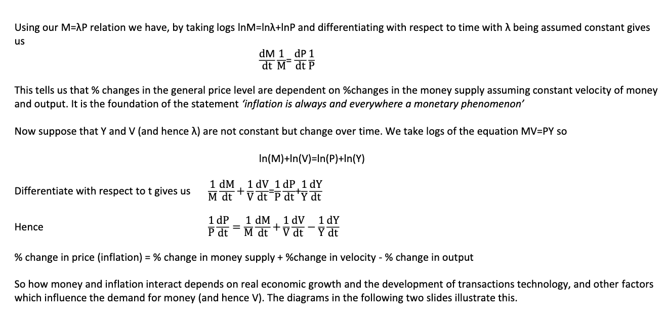
Money and inflation

LOOK AT IMAGE

% changes in the general price level are DEPENDENT on % changes in the money supply assuming a constant velocity of money and output.

% change in price (inflation) = % change in money supply + % change in velocity - % change in output.

So how money and inflation interact depends on real economic growth, the development of transactions technology, and other factors which influence demand for money and V.

What is SEIGNIORAGE. Why do we observe high monetary growth rates and hence high rates of inflation?

The concept of seigniorage is the revenue from the manufacture of notes and coins calculated as the difference between the face value and production cost.

The potential for demand for money to increase as a consequence of rising income and prices provides an opportunity for the government to earn this additional revenue.

Should the additional money generate rising prices then the revenue produced is called the inflation tax. This is because holders of currency see the real value of holdings decline just as if they had been taxed on them.

Seigniorage provides government with a way of funding spending other than using tax.

Countries which issue a currency which is used in other countries have the opportunity to earn seigniorage from the rest of the world. This is the case of the $US.

SO IT IS profit made by a government by issuing currency, especially the difference between the face value of coins and their production costs.

The relation between inflation and nominal interest rates

we derived the expression for the real interest rate, r ≈ i-π or i ≈ r+π. This came from the expression
ln(1+r)= ln(1+i) – ln(1+π) and the approximation came from using ln(1+x)≈x.
Defining (1+r)=𝑒𝑟′
; (1+i)= 𝑒𝑖′
; (1+π)= 𝑒𝜋′
where i, r, and π are the discrete-time nominal interest rate, real
interest rate and rate of inflation while i’,r’,π’ are the equivalent continuous-time rates of change, then i=r+π
With r constant, then any change in the inflation rate should bring forward an identical change in the nominal
interest rate.
But we don’t have perfect predictions of inflation. The Fisher Equation is expressed in terms of expected
inflation:
i = r + π^e where π^e is expected inflation.
This means that the Fisher Equation applies ex-ante, whereas observed data gives ex post real interest rates

e.g. you expect 5% inflation (ex ante) so that with r=2% you set i=7%; if inflation actually is 6% (ex post) with
i=7% then r=1%

Do nominal interest rates follow inflation?

Nominal interest rates follow inflation but usually with a lag.

The Fisher Equation assumes that real interest rates are fixed whereas there has been a decline in recent decades.

The Fisher Equation operates globally with a clear upward relationship but it is not exact due to expectational errors.