ECON 102

Macroeconomics

The study of the structure and performance of the aggregate economy 

Economics

How to evaluate things in economics mainly based on limited or scarce resources, consider what is best, efficient, fair, and rare.

Scarcity

we don’t have unlimited supply

Choice

we decide how to allocate scare resources 

Opportunity Cost

of the next best alternative (if OP cost of A if high, we may want to choose B)

Policies

Aim to incentivize “optimal” behaviour/choice for “best” outcomes

Capitalism

The ownership is in the hands of the private individuals or entities, who control the means of production, distribution, and exchange of goods and services

Command

Government owns the capital (natural resources)

Positive Analysis

What are the effects of the policy (doesn’t have to be factually accurate)

• Making predictions 

Normative Analysis

Should a policy be implemented? -> “TO”

• Value judgements 

Theoretical Models

• Use equations to represent production, behavior, accounting rules, and constraints.

• Graphs to visualize economic relationships (e.g., supply and demand).

• Formalize processes like how resources are allocated or how markets function.

Empirical Tools

• Use data to build models and estimate effects in the real economy.

• Measure magnitudes, such as the impact of policies on output or employment.

• Calibration: Borrow estimates (e.g., labor supply elasticity) from other studies and plug them into models to make predictions.

System of National Accounts (SNA)

• Used to compile accurate and systematic measures of aggregate economic activity of nation or jurisdictional area

• Sets up standardized measurement of macroeconomic variables based on a set of accounting principals.

• One of the common macroeconomic measures generated using the System of National Accounts is GDP.

GDP (Gross Domestic Product)

The market values of all final goods and services produced in an economy during a fixed period of time

• GDP measures "value"

Market Value

• The value of good(s) at market prices

• Price that you see in stores

Measure GDP #1: The Product Approach

Sum all final goods and services produced in the economy at their market value.

Note: final output excludes intermediate production to avoid double counting

Intermediate goods and services

• Those used up in the production of final goods and services within a fixed period of time

• E.x, flour, steel, gold

Value added (of a producer)

• The value of it's output minus the value of it's inputs purchased from other producers

• E.x, Raw products,

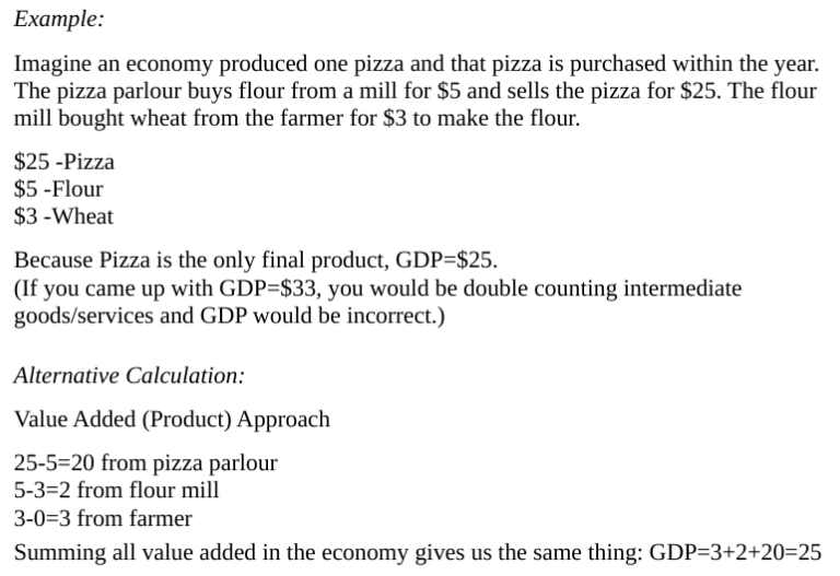
Measure GDP #2: The Expenditure Approach

• Sum all final goods and services purchased in the economy
  

• Pizza example:
  GDP=total spending=1pizza=$25

Income Expenditure Identity

GDP = C + I + G + NX

C= Consumption

I= Investment

G= Government Expenditures

NX= Net Exports

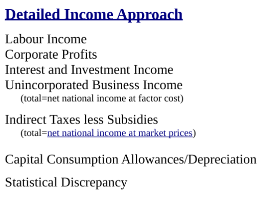
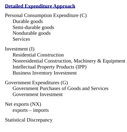
Measure GDP #3: Income Expenditure Identity

• Sum all income received by workers, the government and
  firms (wages, taxes, and profits)

Fundamental Identity of National Income Accounting

Total Production = Total Expenditure = Total Income

No matter which approach we use, product, income or expenditure, we have the same GDP.

Issues of Measurement: GDP

Questions you might ask:

• is GDP comparable across countries?

• does it measure progress accurately?

• what about costs of resources?

• what about costs of pollution (dirty air, water, etc.)?

• do these GDP measures adequately capture quality or value?

• what about happiness?

• should GDP include home production?

• what about unpaid child care?

GNP (Gross National Product)

The total market value of production by all of the national factors of production

GNP: All national (Canadian) workers that are working in other countries

GDP: Production that occurs only in Canada (includes by non-Canadian labour)

• What’s produced in Canada vs. what Canadians produce outside

NFP (Net Factor Payments)

• Income earned abroad by Canadian factors minus income earned in Canada by foreign factors

GNP = GDP + NFP

Savings Identities & Formulas

Saving = current income - current spending

• Change over a period of time

Yd = private disposable income
= the income that households have to spend
= income received from all sources, less taxes

= GDP + NFP + TR + INT – T
where INT is interest on government debt, TR is net transfers, and T is Tax

y = GDP

Yd = Y + NFP + TR + INT – T

Private Saving

Spvt = private disposable income – consumption
Spvt = Yd – C
= (Y + NFP + TR + INT – T) – C

Government Saving

Sgovt = net gov't income – gov't purchases
Sgovt = (T – TR – INT) – G
if Sgovt<0 then gov't has a budget deficit

National Saving

S = Spvt + Sgovt
= (Y + NFP – T + TR + INT – C) + (T – TR – INT – G)
S = Y + NFP – C – G
National Saving = total income – total spending of economy

Recall that Y = GDP = C + I + G + NX, so...
S = Y + NFP – C – G
S = (C + I + G + NX) + NFP – C – G
S = I + NX + NFP

International Components in Savings

CA (Current Account): payments received from abroad less payments made to foreign countries by the domestic economy

CA = NX + NFP
so
S = I + CA

Private Saving Formula

Spvt = I + (- Sgovt) + CA

Saving Vs Wealth (Measurement Type)

Stock Variable: calculated at point in time

Flow Variable: calculated over (within) a period of time

Wealth

The difference between an agent's assets & liabilities

National Wealth
= total wealth of all residents of a country
= domestic physical assets + net foreign assets

net foreign assets
= foreign financial & physical assets – foreign liabilities

Nominal Variable

A variable measured in terms of current market values

Real Variable

A variable measured in terms of a base unit

Accounting for Inflation

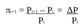
Inflation rate: percentage increase in the price level over a specific period of time

π is the inflation rate
Pt+1 is the price level in period t+1 and
Pt is the price level in period t

How is inflation measured?

Price index: measure of the average level of prices for some specified set of goods and services relative to the prices in a specified base year

• How prices change over time in a spefic region

Three Commonly Used Indices:

1. GDP deflator: price index that measures the overall level of prices of goods & services included in GDP.

GDP deflator = nominal GDP/ real GDP

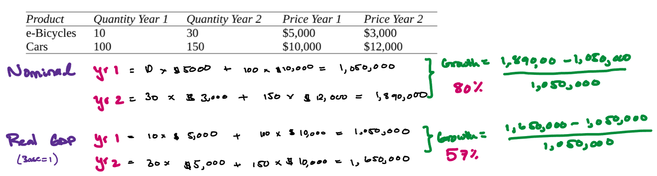
Three Commonly Used Indices:

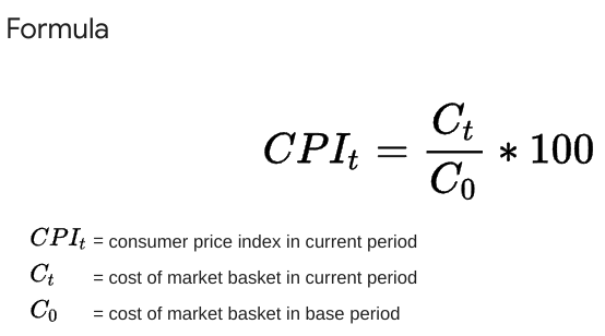
2. CPI (Consumer Price Index): measures changes in prices of subset of consumer goods, a fixed "basket" of goods, relative to a base reference period

Three Commonly Used Indices:

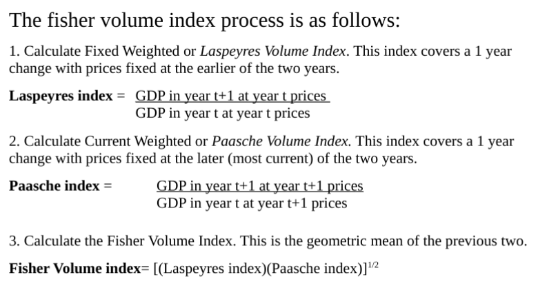
3. Chain Fisher Volume Index: a combination index which changes the base price and chains across time.

• The chained fisher volume index (for a difference of more than1 year) is determined
  by multiplying subsequent indexes.

• Ex/ for year 3 it is: (year 1 to 2)×(year 2 to 3).

• These indexes give the real growth of GDP between the periods indicated, and as
  such Real GDP in subsequent periods should be calculated by multiplying the chain
  Fisher index by the initial (base) year GDP (previous periods are the product of the
  base year GDP and the inverse of the chain fisher index).

Issues with Consumer Price Indexes & “real” GDP

1. Basket becomes outdated
2. Goods may have not existed then & do now
3. Historical measures of real GDP often have to be
recalculated for any comparison

Interest Rates

Interest rate: rate of return promised by a borrower to a lender

Nominal interest rate (i): the rate which is agreed upon between the borrower & lender

Real interest rate (r): the rate at which the real value of the asset (loan value) increases over time

Nominal and Real interest rates Formula

When nominal interest rates and inflation are typically low,
real interest rates can be approximated by

r ≈ i – π

If we are in a period of high inflation and low constant interest rates, is it better to borrow or to lend?

• Since we typically don’t know what inflation will be until the next period is realized, we need to use expected values

• The expected real interest rate is approximated by the nominal interest rate minus expected rate of inflation

i – π^e

Graphing

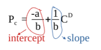
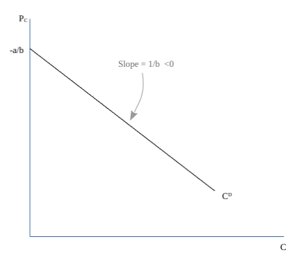
• Carrot Demand: Demand decreases as price rises; downward-sloping line.

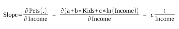
• Pets & Income (Linear): Pets increase steadily with income; more kids raise the intercept.

• Pets & Income (Non-linear): Pets rise with income but slow at higher incomes.

Graphing Pet example

Pets = a + b*Kids + c*ln(Income)

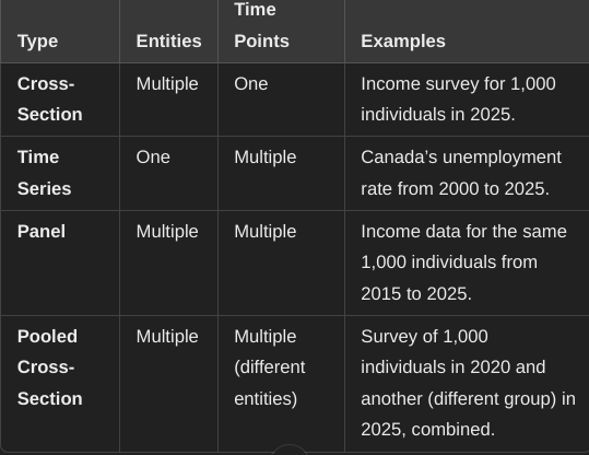
Data Types

• Cross Section: multiple entities at one point in time

• Time Series: one entity across multiple periods of time

• Panel: multiple entities across multiple points of time

• Pooled Cross Section: (multiple entities at one point in time, pooled with another set of entities at a different point in time

Theoretical vs Empirical

Theoretical Analysis (Theory)

• Formalizes economic theories with mathematical expressions.

• Focuses on behavior, constraints, and institutional rules.

• Produces testable predictions through solutions to equations.

• Goal: Use logic to predict how the economy should behave.

Empirical Analysis (Data)

• Uses data, statistics, and mathematics to test hypotheses.

• Estimates the magnitude of relationships suggested by theory.

• Focuses on observing real-world patterns and verifying predictions.

Model Classifications

Treatment of Information
e.g. full information vs missing or asymmetric information

Time Dimension
e.g. static vs dynamic

Treatment of State Dependency
e.g. deterministic vs stochastic

Type of Agent(s)
e.g. representative agent vs more than one type of agent

Scope
e.g. Partial vs General Equilibrium

Market Functionality
e.g. Market clearing vs non-clearing models

Which class of models would be more appropriate to study business cycle or recession duration, Static or Dynamic?

• Modern macroeconomic models are often dynamic, incorporating stochastic and general equilibrium frameworks, while some non-equilibrium models like search & matching are also widely used.

• The IS-LM model, though previously popular for teaching, is criticized for lacking dynamic features and realistic market treatments

Model Elements

Variable (take on different values and they vary)

• refers to an item (e.g. price, interest rates,
  consumption, investment, GDP) that can take on different
  possible values

• Variables represent both the inputs to models, and the outputs
  from models

• Error terms (u)

Endogenous: determined within the model (most variables)
Exogenous: determined outside of the model (right-hand side)

e.x, Wheat→ the output is exogenous

What goes into the making of wheat (labour, sun, soil, etc.) → endogenous

Parameters: Lower Case

• characterize the strength and direction of relationships between variables. (the a, b, g’s and α, β, ɣ’s)

• In theoretical analysis, parameters are sometimes calibrated, but they can also be estimated, as they are in empirical analysis

• Estimation is conducted by applying the model to data, to determine (and test) the predicted relationship between variables

Building Macroeconomic models

• Incorporating several components of the economy (relationship between variables of interest)

• Components of economic models are often framed in relation to markets (e.g., labour, goods, financial, etc.), market participants (e.g., buyers, sellers, regulators), & or outcomes (e.g., prices, quantities, aggregates, and distributions)

Production

processes or production functions are a key component that helps us understand firms’ supply decision (how much they wish to sell in the goods market), but also firms’ demand for inputs (e.g. labour and capital) in their respective markets

Factors of production: inputs such as capital, labour, raw materials, land and energy utilized by the producers in the economy

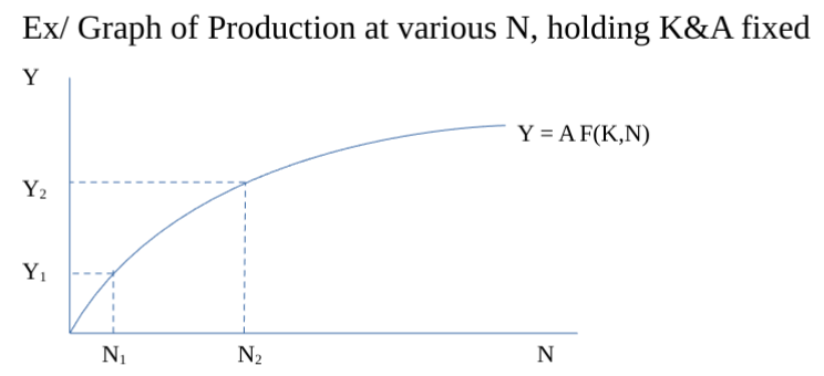
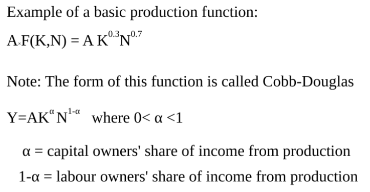
Aggregate Production Function (Basic Example)

Y = A x F(K,N)

Y=real output produced
A=a multiplicative productivity effect
K=quantity of capital used
N=the number of workers employed
F=a function specifying how much output is
derived from given quantities of input K & N

• Non-linear due to dimishing returns (more production results in smaller increases in outputs)

• Never slope down

Firms objective: Profit Maximization

• Major factor in firm decsians making to determine quanities of input and output

Profit maxing quantities of N & K determined by:

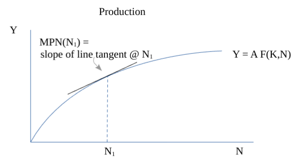
*Marginal Product of Labour (MPN)
= the increase in output resulting from a one unit increase in labour
= ∆Y/∆N

*Marginal Product of Capital (MPK)
= the increase in output resulting from a one unit increase in capital
= ∆Y/∆K

*Relative Prices

TFP – Total Factor Productivity

A = Measuring Productitivty

A is generally calculated using the “known” factors of Y and F(K,N)

if Y=A×F(K,N) then A = Y / F ( K , N )

The level of A is important in firms’ decision making, and factor markets, because it influences MPK and MPN

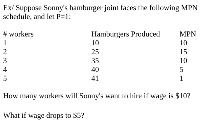
Labour Demand

* To determine how many workers to hire, firms need to compare the costs and benefits of hiring an additional worker

What are the benefits of hiring on more worker?

MPN x P = MRPN

MRPN is Marginal Revenue Product of Labour
What is the cost of hiring an added worker?

nominal wage: the wage that is paid to worker

Hiring Rule (Profit Maximizing Decision)

firm will continue to hire so long as MRPN ≥ W Firms maximize profits by hiring until

MRPN = W

How do we know this maximizes profits?

Profits = revenue – costs = P x Q – N x W
Q is quantity produced by the production process, e.g., A*F(K,N)

• W=Marginal Cost

• MRPN is Marginal Benefit

• Profit maximization occurs where MB=MC

Hiring rule in real terms

MPN = w

w = W/P = real wage

real wage: nominal wage divided by price level

• Economic models often discuss outcomes in real terms

• Labour demand can be written as function of real wages in a
  complex or simple way, e.g.

  N^D=f(w) where f'(w)<0

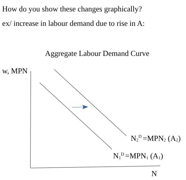
Labour Demand Curve

Labour demand curve: the amount of workers a firm will wish to hire at given wages

Factors that Shift Labour Demand Curve

1. Beneficial productivity shock
2. Higher capital stock

Aggregate Labour Demand: the sum of all labour demands of all firms in the economy

• e.g. 100 firms like Sonny’s would mean an aggregate labour demand of ND=500-20w
  (or as we graph it w=25-ND/20). Of course, a more complex function would
  incorporate more depending on the research question e.g. ND=f(A,K,w

Labour Supply

Labour Supply: labour the worker is willing to supply

Labour Supply Curve

Labour Supply Curve: the labour the worker is willing to supply at given wages
Aggregate Labour Supply: sum of all individual labour supply
Aggregate Labour Supply curve: sum of all labour that workers are willing to supply given at wages

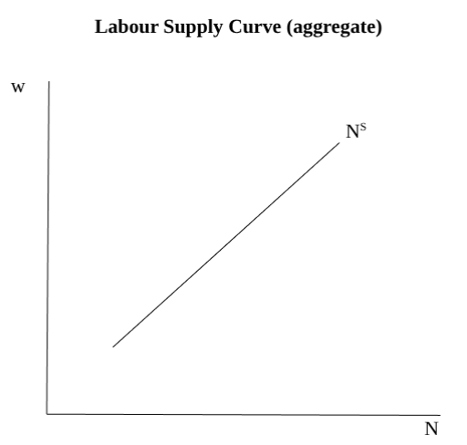
Factors that Shift Labour Supply Curve

1.Wealth: increase in wealth will decrease the labour supply
2.Expected future real wage: increase in E[wf] will decrease the labour supply
3.Population: increase in population will increase labour supply
4.Participation rate: Increase in LFP will boost labour supply

Labour Market Equilibrium

In this simple, market clearing, labour market example, equilibrium occurs when ND=NS

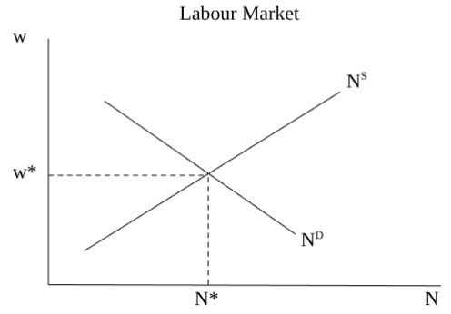
Potential Output

Labour Market Equilibrium and Potential Output What the economy actually produces is typically called output (or national output or national income or actual output), and is denoted by Y

Full Employment Output (or Potential Output): is a measure of what the economy would produce if all resources were fully employed, sometimes denoted by Y* or FE

Full-Employment level of employment: the equilibrium level of employment, N (or N*, or N)

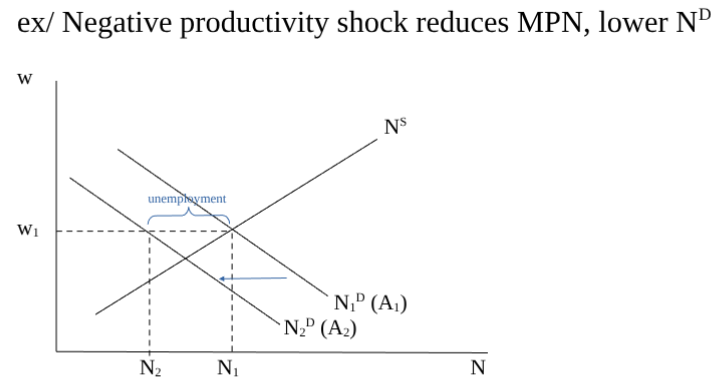
Sticky wage models

Can be graphed similar to our market clearing model, but wages “stick” and do not adjust quickly to clear the market

Institutional Factors: Wage floors and/or negotiated contracts might keep wages above market clearing levels

Search & Matching Framework

• Job search: Workers and firms take time to find suitable matches.

• Match dynamics: Jobs are temporary; workers or firms may part ways.

• Unemployment: Constant due to search time and job turnover.

flows in = flows out

flows in: # of matches M(U,V)

• U is the number of unemployed and V is number of vacancies (job postings)

flows out: δE → matches destroyed

• E is # employed

M(U,V) = δE

Key Labour Market Terms/Measures

Employed: worked full-time or part-time during past week

Unemployed: without work during past week and actively looked for work during past 4 weeks. Excludes full-time students

Not in the Labour Force: not working during past week, and not looking for work in past 4 weeks

Labour Force (LF) = Employed + Unemployed

Participation Rate = Labour Force/working age population

Unemployment Rate (R4) = Unemployed/Labour Force

Employment Ratio (Rate) = Employed/working age population

Types of Unemployment

1. Frictional: Workers are unemployed briefly when changing jobs

2. Structural: Longer term unemployment which may result from poor
capabilities, or from changes in economy that shift demand from one industry/skill/area to another

3. Cyclical: Occurs as the economy fluctuates around full- employment level

Natural Rate of Unemployment: unemployment due to frictional and structural causes

Issues in Measuring Unemployment

Discouraged workers: people become discouraged by not finding a job and stop searching

Underemployment: people may be able to find part time, but wish to work full time

Long-Term Unemployment: people unable to find jobs for longer periods of time

Measures of Unemployment

R1: Proportion of LF out of work for 1 year or more
R2: Proportion of LF out of work for 3 months or more
R3: Unemployment Rate per U.S. definition
R4: Official Unemployment Rate
R5: Includes discouraged workers
R7: Includes involuntary part-time workers

Factors that can influence changes in unemployment

1. Participation rate changes
2. Structural changes in the economy
3. Policy Changes that influence incentives
4. Hysteresis
*skills and mis-match
*insider/outsider theory