Transformation

Lesson 4

Trivial

re-expression of values, but no impact on the shape of distribution

Multiplication of constant

world_density$DensityTimes4 <- 4*(world_density$Density)

• This operation scales the values of the density by a constant factor, affecting the magnitude but not the overall distribution shape.

Addition of constant

world_density$DensityPlus100 <- 100+world_density$Density]

• This operation shifts the values of the density by a constant amount, altering the location of the distribution without changing its shape.

Nontrivial

Re-expression of values that changes the shape of distribution

Basic power transformation

A method that raises values to a specified power, altering the shape of the distribution and potentially stabilizing variance.

Alternative power transformation

A technique that applies a different power to values, aiming to achieve a more normal distribution and stabilize variance across data.

All of the graphs go through (1, 0) and have the same slope at that point.

All of the curves are increasing in x.
Thus, the order of data are preserved.

If p > 1

The graph is concaved up, and as p moves away from 1, the curve becomes more curved, which means that the concavity increases.

The transformation will expand the scale more for large xx than for small xx

If p < 1

the graph is concaved down

the transformation will compress the scale more for large xx than for small xx.

if p = 1

the graph is linear

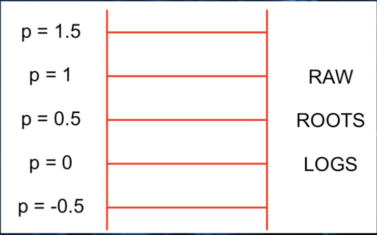
Tukey’s Ladder of power

Create a stemplot

stem(df$attribute)

Create histogram

ggplot(CO2emissions, aes(CO2emissions)) + geom_histogram(color = "blue", fill = "white", bins=15) + geom_density(aes(x = CO2emissions)) + theme_classic(base_size = 15) + labs(x = "CO2emissions")

letter values

lvals ← lval(df$attribute); lvals

Symmetric Data

the mids does not show any trend

Right skewness

the mids are increasing and the tailis on the right side.

Left skewness

the mids are decreasing and the tail is on the left.

Plotting the mids

lvals %>% mutate(LV = 1:8) %>% ggplot(aes(LV, mids)) + theme_classic(base_size = 25) + geom_point()

getting the square root of the attribute you want t re-express

df$attribute ← sqrt(df$attribute)

Hinkley’s quick method

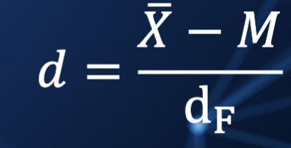
Hinkley code

hinkley(df$attribute)

Inspect the mids

logval ← lval(df$attribute) logva

Symmetry Plot

plot showing the symmetry of a batch

STEPS

1. Arrange the values, from y₍₁₎, y₍₂₎, y₍₃₎,…, y_(n).

2. If M is the median, then plot

   𝒖𝒊 = 𝒚(𝒏)𝟏+𝒊) − 𝑴 on the vertical axis, versus
   𝒗𝒊 = 𝑴 − 𝒚(𝒊) on the horizontal axis
   for 𝑖 = 1, 2 , 3, ... 𝑛/2 if 𝑛 is even and (𝑛 + 1)/2 if 𝑛 is odd.

3. Add the line 𝒖 = 𝒗 to the graph as the line of symmetry

Symmetry Plot code

example ← c(4, 5, 6, 7, 8, 9, 9, 10, 14, 18, 19) stemplot(example)

Editing a function in R (default)

edit(function)

Editing a function in R (editing the symplot)

edit(symplot)

Modify the symplot function

symplot ← (paste the script you just highlighted)

Comparison of re-expressed data

boxplot(data.frame(CO2emissions$CO2emission,
CO2emissions$sqrtCO2,
CO2emissions$logCO2,
CO2emissions$recrootCO2,
CO2emissions$CO2p))