Chapter 5

🧠 Study Guide: 5.1 Basic Concepts CPU Scheduling

📝 Overview
• CPU scheduling is essential in multiprogrammed systems.
• It ensures the CPU is utilized effectively by switching between processes.
• Threads (not whole processes) are actually scheduled, but terms are often used interchangeably.
• A process runs on a CPU core, and multiple cores enable parallel execution.

🔁 Basic Concepts

• Single core systems can run one process at a time.

• Multiprogramming keeps multiple processes in memory to avoid idle CPU time.

• The OS switches CPU from waiting processes to ready ones.

  

🔄 CPU I/O Burst Cycle

• Process execution alternates between CPU bursts and I/O bursts.
• Typical execution:
CPU burst → I/O burst → CPU burst → … → Terminate
• I/O  bound programs: many short CPU bursts
CPU bound programs: fewer, longer CPU bursts

• Burst durations often follow exponential/hyperexponential distributions.

🧮 CPU Scheduler

• Picks the next process to run from the ready queue.
• The ready queue can be FIFO, priority queue, tree, or unordered list.
• The entries in the ready queue are Process Control Blocks (PCBs).

⚖️ Preemptive vs. Nonpreemptive Scheduling

Preemptive Nonpreemptive
OS can take CPU away from running process Process keeps CPU until it finishes or blocks
Used by most modern OSes Simpler but not ideal for real

⚙️ Dispatcher

• Transfers control of the CPU to the selected process.
• Performs:
○ Context switch
○ Switching to user mode
○ Jumping to user program entry point
⏱️ Dispatch latency: Time to stop one process and start another.

📊 Context Switching

• Tracked via tools like vmstat and /proc/[pid]/status
• Two types:
○ Voluntary: process blocks (e.g., I/O)
○ Nonvoluntary: process preempted (e.g., time slice expired)
Example:
vmstat 1 3
cat /proc/2166/status

🧩 Common Issues

• Race conditions if processes share data and get preempted mid

• Preemptive kernels must guard shared data (use locks, disable interrupts).

• Nonpreemptive kernels are safer but less responsive for real-time.

  

🧠 Study Guide: 5.2 Scheduling Criteria

📝 Overview

• CPU scheduling algorithms have different properties, and choosing the right one depends on several factors.
• The criteria used for comparison significantly influence the decision about which scheduling algorithm is optimal in a given scenario.

🎯 Key Scheduling Criteria

These criteria are used to assess how effective a CPU scheduling algorithm is:
1. CPU Utilization
○ Definition: Measures how well the CPU is used.
○ Goal: Maximize CPU usage.
○ Range: Ideal range is 40% to 90% (depending on system load).
○ Real world measurement: Can be measured using commands like top in Linux/macOS/UNIX.

1. Throughput

   • Definition: The number of processes completed per unit of time.

   • Goal: Maximize the throughput (the more processes, the better the system's efficiency).

   • Consideration: Throughput is higher for systems that deal with short processes, whereas long-running processes may reduce throughput.

2. Turnaround Time

   • Definition: The total time taken for a process to execute from submission to completion.

   • Formula:
     Turnaround Time = Waiting Time + CPU Time + I/O Time

   • Goal: Minimize turnaround time to ensure faster completion of processes.

   • Impact: Affects how long a user must wait for a process to finish.

3. Waiting Time

   • Definition: The amount of time a process spends in the ready queue waiting to get CPU time.

   • Formula:
     Waiting Time = Turnaround Time _ (CPU Time + I/O Time)

   • Goal: Minimize waiting time to make the system more responsive.

   • Impact: Longer waiting times can delay process execution and reduce system performance.

4. Response Time

   • Definition: The time it takes for a system to start responding after a request is made.

   • Goal: Minimize response time for interactive systems.

   • Important: For interactive systems, such as PCs, response time is more important than turnaround time. It measures how quickly a user receives feedback from the system.

   • Impact: Quick response time is crucial for user satisfaction in interactive environments.

⚖️ Optimization Goals

• Maximization Goals:
○ Maximize CPU Utilization and Throughput to make the system as efficient as possible.
• Minimization Goals:
○ Minimize Turnaround Time, Waiting Time, and Response Time to improve the user experience.
• Special Cases:
○ Sometimes, minimizing the maximum response time is more critical than average values, particularly in systems where guaranteed good service for all users is important (e.g., real

📊 Variance in Response Time (Interactive Systems)

• In interactive systems, variance in response time can be more important than simply minimizing average response time.
○ Reason: Predictable behavior is often preferred over systems that may be faster on average but are erratic in their responsiveness.
○ Goal: Aim for consistency in response times to ensure users don’t experience sudden slowdowns.

🧠 CPU Scheduling Key Concept

CPU scheduling determines which process in the ready queue gets the CPU when it becomes available. For this section, we assume a single

1. First Come, First Served (FCFS)

• Type: Nonpreemptive
• Mechanism: Processes executed in the order they arrive.
• Cons: Long average waiting time, convoy effect.
• Fair but not optimal.

2. Shortest Job First (SJF)

• Type: Preemptive or Nonpreemptive
• Mechanism: Process with the shortest next CPU burst is scheduled.
• Optimal for minimizing average waiting time.
• Requires prediction of burst time using exponential averaging.

3. Round Robin (RR)

• Type: Preemptive
• Mechanism: Each process gets a fixed time quantum.
• Best for time sharing systems.
• Balance between responsiveness and context

4. Priority Scheduling

• Type: Preemptive or Nonpreemptive

• Mechanism: Process with the highest priority gets the CPU.

• Can suffer from starvation.

• Aging can be used to prevent indefinite blocking.

5. Multilevel Queue Scheduling

• Type: Can be preemptive or non-preemptive

• Mechanism:

  • Separate queues for each priority or process type.

  • Fixed priority scheduling between queues: higher-priority queues are served first.

  • Round robin may be used within each queue.

• Example Queues:

  1. Real-time

  2. System

  3. Interactive

  4. Batch

CPU is always allocated to the highest non-empty queue.

⏱ Time Slicing Among Queues:

• CPU time is divided (e.g., 80% for interactive, 20% for batch).

• Can use different scheduling strategies per queue (e.g., RR for one, FCFS for another).

6. Multilevel Feedback Queue Scheduling

• Type: Preemptive
• Mechanism:
○ Like multilevel queue, but processes can move between queues.
○ Shorter jobs stay at higher priorities; CPU heavy jobs are demoted.
○ Aging allows long waiting processes to move up in priority.
Example Setup:
• Queue 0: RR, quantum = 8 ms
• Queue 1: RR, quantum = 16 ms
• Queue 2: FCFS
• New processes start in queue 0 → if not finished, demoted to next queue.
🔄 Feedback Logic:
• Long CPU burst → demotion
• Long wait → promotion (aging)
⚙️ Configuration Parameters:
1. Number of queues
2. Scheduling policy for each queue
3. Rules for promotion/demotion
4. Rules for initial queue assignment
Most flexible but most complex to configure. Can emulate other algorithms.

📊 Comparison Table

📊 Comparison Table-

Algorithm	Preemptive	Starvation Risk	Best For	Fairness
FCFS	No	No	Simple systems	Low
SJF	Optional	Yes	Batch systems	Medium
RR	Yes	No	Interactive systems	High
Priority Scheduling	Optional	Yes	Importance-based scheduling	Varies
Multilevel Queue	Yes	Yes (fixed)	Class-based separation	Medium
Multilevel Feedback Queue	Yes	No (with aging)	General-purpose, adaptive	High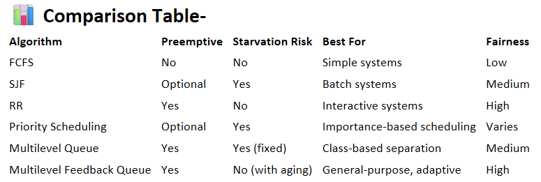

🧠 5.4 Thread Scheduling

🌐 Overview

• In modern OSes, threads not full processes are scheduled.
• Kernel level threads are managed by the OS scheduler.
• User level threads are managed by a thread library (e.g., Pthreads).
• To execute, user level threads must be mapped to kernel level threads or LWPs (Lightweight Processes).

🧩 1. Process Contention Scope (PCS)

• Competition among threads in the same process
• Managed by the thread library, not the OS
• Typical in:
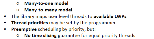
- Many-to-one model

• Many-to-many model

• The library maps user level threads to available LWPs

Thread priorities may be set by the programmer

Preemptive scheduling by priority, but:

No time slicing guarantee for equal priority threads

🌍 2. System Contention Scope (SCS)

• Competition among all threads system wide
• Managed by the OS kernel
• Typical in:
○ One to one model
○ Examples: Linux, Windows
• Only SCS is used in one to one threading systems

🔧 Pthread Scheduling

The POSIX Pthreads API supports specifying contention scope during thread creation.
✨ Contention Scope Options
• PTHREADSCOPEPROCESS → PCS (librarylevel)

• PTHREAD_SCOPE_SYSTEM → SCS (OS-level)

⚙️ API Functions

int pthreadattrsetscope(pthreadattrt *attr, int scope);
int pthreadattrgetscope(pthreadattrt *attr, int *scope);
• attr: pointer to thread attributes
• scope: value to set or retrieve
○ PTHREADSCOPESYSTEM
○ PTHREADSCOPEPROCESS
• Returns 0 on success, nonzero on error

🛠️ Example Workflow

1. Check current contention scope with pthreadattrgetscope
   2. Set contention scope with pthreadattrsetscope
   3. Create threads that inherit the defined scope

🔒 System Limitations

• Not all systems allow both scopes
• Linux and macOS: Only allow PTHREADSCOPESYSTEM

🧠 5.5 MultiProcessor Scheduling

🌐 Introduction

In multii-core systems, scheduling becomes more complex than on a single core CPU. Scheduling must now consider multiple CPUs/cores and how to efficiently balance threads across them.

Types of Multiprocessor Systems:

• Multicore CPUs = Multiple cores on one chip

• Multithreaded cores = Each core supports multiple threads

• NUMA systems = Memory access time depends on processor-memory proximity

• Heterogeneous Multiprocessing (HMP) = Cores have different power/performance profiles (e.g., ARM big.LITTLE)

🧭 Approaches to Multi Processor Scheduling

🔁 1. Asymmetric Multiprocessing (AMP)
• One core does all scheduling and I/O (the "boss")
• Simpler, avoids race conditions
• Downside: Becomes a bottleneck
🔄 2. Symmetric Multiprocessing (SMP)
• Each processor self schedules from the ready queue
• Two strategies:
○ Common ready queue (shared, needs locks)
○ Per processor queues (private, avoids contention) ✅ Most common

🧠 Multicore Processors & Scheduling Challenges

🏃‍♂️ Memory Stalls
• CPUs often wait for memory (e.g., cache misses)
• Can waste up to 50% of CPU time
🧵 Chip Multithreading (CMT)
• Each core has multiple hardware threads
• OS sees each thread as a logical CPU
• When one thread stalls, another can run
🧠 Intel Hyper Threading (aka SMT)
• 2 threads/core (e.g., Intel i7)
• Oracle SPARC: 8 threads/core

🪄 Types of Multithreading

Type Description
Coarse grained Switch threads only on long stalls; expensive context switch
Fine grained Switch threads every cycle; requires special hardware, but less overhead
🎛️ Two Levels of Scheduling
1. OS Scheduling: Choose which software thread runs on which hardware thread
2. Hardware Scheduling: Choose which hardware thread runs on a core (e.g., round

⚖️ Load Balancing

Purpose:
• Prevent some processors from being idle while others are overloaded
Works Best On:
• SMP systems with per-processor queues

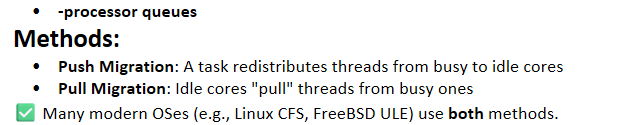
Methods:

• Push Migration: A task redistributes threads from busy to idle cores

• Pull Migration: Idle cores "pull" threads from busy ones

✅ Many modern OSes (e.g., Linux CFS, FreeBSD ULE) use both methods.

📍 Processor Affinity

Why It Matters:
• Threads leave cached data on a CPU
• Moving them causes cache repopulation (costly)
Types of Affinity:
Type Description
Soft Affinity OS tries to keep thread on the same CPU but not guaranteed
Hard Affinity Application/OS sets specific CPUs a thread must run on
• Linux supports both via sched_setaffinity()
NUMA Systems
• Memory is closer to specific CPUs
• OS can optimize memory placement + scheduling for performance

🔀 Heterogeneous Multiprocessing (HMP)

What Is It?
• CPUs with different core types (e.g., ARM big.LITTLE)
• Some are high power, some low power
Why Use It?
• Save battery power
• Use big cores for short, intensive tasks
• Use LITTLE cores for long

🧠 Key Concepts

🎯 1. Real Time Systems:
• Soft Real Time:
○ No guarantee of meeting deadlines, but real-time tasks are given priority.

• Hard Real Time:

  • Deadlines must be met. Missing a deadline = failure.

⏱️ 2. Latency in Real Time Systems

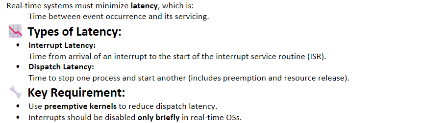
Real-time systems must minimize latency, which is:

Time between event occurrence and its servicing.

📉 Types of Latency:

• Interrupt Latency:
  Time from arrival of an interrupt to the start of the interrupt service routine (ISR).

• Dispatch Latency:
  Time to stop one process and start another (includes preemption and resource release).

🔧 Key Requirement:

• Use preemptive kernels to reduce dispatch latency.

• Interrupts should be disabled only briefly in real-time OSs.

  

🧾 3. Priority Based Scheduling

• Essential for both soft and hard real time systems.
• Must support preemption.
• High priority process interrupts a lower one.
OS Examples:
• Windows: Real time priorities 16 31.
• Linux & Solaris: Similar prioritization.
✅ Enables soft real time support. ❌ Doesn’t guarantee hard deadlines — for that, we need special algorithms.

📅 4. Periodic Real Time Tasks

Each periodic task is defined by:
• Processing Time (C)
• Deadline (D)
• Period (T)
Relationship: 0 ≤ C ≤ D ≤ T
Admission

📊 5. Real Time Scheduling Algorithms

5.1 📉 Rate Monotonic Scheduling (RMS)
• Static priority: Shorter period = higher priority.
• Preemptive
• Assumes constant CPU burst times.
🔧 Limitations:
• Not all task sets are schedulable.
• CPU utilization bound:
n(2^(1/n) minus 1) (for n processes)
With 2 tasks, ~83% max CPU utilization.

5.2 ⏰ Earliest Deadline First (EDF)

• Dynamic priority: Earlier deadline = higher priority.
• Can schedule tasks with variable bursts and deadlines.
• Optimal in theory: Can achieve 100% CPU utilization.
🔍 In practice: Context switching and overhead limit efficiency.

5.3 ⚖️ Proportional Share Scheduling

• CPU time divided into shares.
• A process with s shares out of T total gets s/T of CPU time.
🔒 Admission Control ensures share guarantees.
Example:
• Process A: 50 shares
• Process B: 15 shares
• Process C: 20 shares
→ 85/100 allocated, no room for a new 30 share request.

📚 6. POSIX Real Time Scheduling

• SCHEDFIFO: ○ First come, first served. ○ No time slicing for equal priority threads. • SCHEDRR:
○ Round robin with equal priority.
○ Includes time slicing.
• SCHEDOTHER: ○ System dependent; not specified by POSIX. 🔧 API Functions: • pthreadattrgetschedpolicy() • pthreadattr_setschedpolicy()
Used to get/set scheduling policies on threads.

✅ Summary Table

Feature Soft RT Hard RT
Deadline Guarantee ❌ ✅
Preemptive Kernel Needed Recommended Required
Interrupt/Dispatch Latency Should be low Must be low
Admission Control ❌ ✅
Common Algorithms Priority, RR RMS, EDF, Proportional

🔧 Section 5.7: Operating System Examples

🌱 General Overview

• This section examines process (thread/task) scheduling in:

  • Linux

  • Windows

  • Solaris

• Key focus: kernel thread scheduling, load balancing, priority classes, and responsiveness.

  

🐧 Linux Scheduling

⏩ History and Evolution
• Pre 2.5: Traditional UNIX like scheduler; poor SMP (Symmetric Multiprocessing) support.
• 2.5 Kernel: Introduced O(1) scheduler (constant time scheduling).
○ Improved SMP, processor affinity, load balancing.
○ Poor response time for interactive tasks.
• 2.6.23 Kernel: Replaced by Completely Fair Scheduler (CFS).

⚙️ CFS (Completely Fair Scheduler)

🔸 Key Concepts:
• Schedules tasks fairly, based on virtual runtime (vruntime).
• No fixed time slices. Uses a targeted latency interval.
• Task with smallest vruntime is selected next.
🔸 Priority:
• Based on nice values (neg20 to +19); lower is higher priority.
• Nice value affects CPU proportion, not direct priority.
🔸 vruntime:
• Measures how long a task has run (adjusted by nice value).
• Stored in red black tree for fast access (leftmost = next to run).
🔸 Load Balancing:
• NUMA aware with scheduling domains.
• Minimizes thread migration.
• Hierarchical balancing (within core → socket → NUMA node).
🔸 Real Time Scheduling:
• Uses POSIX policies (e.g., SCHEDFIFO, SCHEDRR).
• Priority range:
○ Real time: 0 to 99
○ Normal: 100 to 139 (derived from nice values)

🪟 Windows Scheduling

⚙️ Scheduler Overview
• Uses preemptive, priority based scheduling.
• Scheduler = Dispatcher.
• Runs highest -priority thread.

• Two priority classes:

  • Real-time (16 to 31)

  • Variable (1 to 15)

🧱 Thread Priorities

🔸 Priority Classes (Set via API):
• IDLEPRIORITYCLASS
• BELOWNORMALPRIORITYCLASS • NORMALPRIORITYCLASS (default) • ABOVENORMALPRIORITYCLASS
• HIGHPRIORITYCLASS
• REALTIMEPRIORITYCLASS
🔸 Relative Priorities:
• IDLE, LOWEST, BELOWNORMAL, NORMAL, ABOVENORMAL, HIGHEST, TIMECRITICAL 🔸 Example: HIGHPRIORITYCLASS + ABOVENORMAL → priority 14
🔸 Thread behavior:
• Quantum expiration → priority reduced (but not below base).
• Boosted on return from wait (e.g., I/O wait gets higher boost).

🖥️ Foreground Boost

• Foreground processes get longer time quantum (usually 3×) to improve responsiveness.

🧵 UMS (User Mode Scheduling)

• Introduced in Windows 7.
• Allows apps to schedule threads in user space.
• Successor to fibers (less efficient due to shared thread environment block).

🧠 Multiprocessor Scheduling

• Threads assigned ideal processor and SMT sets to reduce cache penalties.
• Logical processor allocation rotates seed to distribute load:
○ Process 1: 0, 2, 4, 6
○ Process 2: 1, 3, 5, 7

☀️ Solaris Scheduling

📊 Scheduling Classes
1. Time Sharing (TS) (default)
2. Interactive (IA)
3. Real Time (RT)
4. System (SYS)
5. Fair Share (FSS)
6. Fixed Priority (FP)

📈 Time Sharing (TS) & Interactive (IA)

• Multilevel feedback queue.
• Inverse priority to quantum relation:
○ Higher priority → smaller quantum.
○ Lower priority → longer quantum.
• Boosted priority when waking from sleep (e.g., I/O wait).

🔝 Other Classes

• RT: Highest priority, used sparingly.
• SYS: Used by kernel threads; priority doesn't change.
• FP: Priority fixed, not adjusted dynamically.
• FSS: Uses CPU shares instead of priorities (per project).

🔁 Global Prioritization

• Class-specific → global priority mapping.

• Scheduler picks highest global priority to run.

• Uses round robin for same-priority threads.

  

📌 Quick Comparison Table

Feature Linux (CFS) Windows Solaris
Scheduling Basis vruntime (fairness) Priority based (dispatcher) Class based with global priority
Real Time Support POSIX (0 to 99) Real time class (16 to 31) Real time class (highest priority)
Default Class CFS (normal tasks) NORMALPRIORITYCLASS Time Sharing (TS)
Thread Storage Red black tree Priority queues Multilevel feedback queue
Priority Boost I/O bound tasks favored Wait time & foreground boost Boost on return from I/O sleep
SMP Support Yes, NUMA aware domains Ideal processor & SMT sets Not emphasized

🔍 5.8 Algorithm Evaluation

📌 Purpose of Algorithm Evaluation
• To choose the best CPU scheduling algorithm for a specific system.
• Many algorithms exist (FCFS, SJF, RR, etc.), each with different goals and trade offs.
• Selection depends on performance criteria such as:
○ CPU Utilization
○ Response Time
○ Throughput
○ Turnaround Time
○ Waiting Time

⚙️ Step 1: Define Evaluation Criteria

• Choose what's most important for your system:
○ Maximize CPU utilization under constraint (e.g., response time < 300ms)
○ Maximize throughput with conditions (e.g., turnaround time ∝ execution time)

📊 1. Deterministic Modeling

• Analytical method with a predefined workload.
• Simple & fast but works for specific scenarios only.
🧠 Example:
• 5 Processes, All Arrive at Time 0
Process Burst Time
P1 10 ms
P2 29 ms
P3 3 ms
P4 7 ms
P5 12 ms
✅ Results:
• FCFS: Avg wait time = 28 ms
• SJF: Avg wait time = 13 ms
• RR (Quantum = 10ms): Avg wait time = 23 ms
🧠 Conclusion:
• SJF gives the minimum average waiting time.
• Limitations: Works only for known workloads; not generalizable.

📈 2. Queueing Models

• Uses mathematical modeling based on probability distributions:
○ CPU burst times: typically exponential
○ Arrival rates: modeled using Poisson/exponential
• Models the system as a network of queues (CPU, I/O)
📏 Key Formula: Little’s Law
L = λ × W
• L: Average number of processes in the queue
• λ: Average arrival rate (e.g., 7 processes/sec)
• W: Average waiting time
🧠 Pros:
• Theoretical framework for comparing algorithms.
🚫 Cons:
• Makes simplifying assumptions.
• May use unrealistic distributions.

💻 3. Simulations

• Uses a simulated model of a system with a virtual clock.
• Driven by:
○ Random distributions (exponential, Poisson, etc.)
○ Trace files (actual recorded events from real systems)
📈 Example Metrics Tracked:
• CPU utilization
• Waiting time
• Throughput
🧠 Pros:
• More realistic than deterministic modeling or math.
• Trace files provide accurate, real world evaluations.
🚫 Cons:
• Time consuming, requires lots of compute and storage.
• Complex to design and debug.

🧪 4. Implementation

• Most accurate method: implement the algorithm on a real system.
• Test under real workloads and track performance.
🧠 Pros:
• Real world accuracy.
• See how users and programs interact with the scheduler.
🚫 Cons:
• Expensive & time intensive
• Requires modifying OS code, regression testing, etc.
• Behavior may change due to:
○ Users trying to game the scheduler
○ Different application needs

📚 Summary Table

Method Realism Complexity Use Case
Deterministic Model Low Easy Teaching, examples
Queueing Models Medium Moderate Theoretical comparison
Simulation High High Realistic evaluation, trace