S301 Key definitions, formulae and papers

5 threats to internal validity

• Omitted variable bias - omitted variable is a determinant of Y correlated with at least one regressor

  • Solution - IVs, include omitted variable if measurable, FEs, or run a RCT

• Functional form bias - i.e. forgetting an interaction term

  • Use the right nonlinear specification

• Errors in variables bias - measurement error of some kind

  • Solutions: better data, model the error process specifically, use IVs

• Sample selection bias - selection process influences data availability and is related to dependent variable

  • change selection procedure, model it or use an RCT

• Simultaneous causality bias - Y causes X and X causes Y, so impossible for either to be exogenous

  • Use and RCT, model both directions of causality completely or use IVs

Identifying bias from errors-in-variables under certain assumptions

Potential outcomes: two ways of viewing the lack of a counterfactual for each observations

1. Missing data - don’t observe the outcome without treatment for someone who received it

2. Selection bias - inference can’t be made because those who receive treatment and those who don’t are different in some systematic way

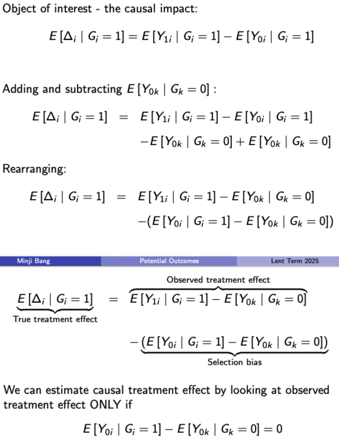
Illustrating selection bias in potential outcomes framework (remember that the initial causal impact term includes a non-observable counterfactual E[Y(0i) | G(i) = 1]

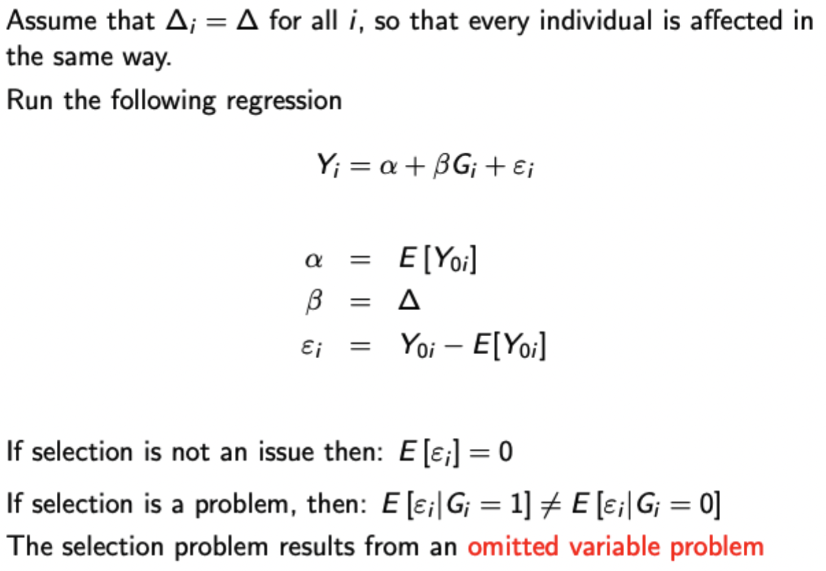
Selection bias in regression context

Issues with internal validity in RCTs

• Noncompliance: randomisation breaks down in some way:

  • Attrition (dropouts) particularly an issue for LR effects

  • Movement across assignment types

  • Substitution bias may occur if individuals in the control group obtain some substitute for the treatment outside the scope of the study.

Intent to treat

Estimator for the ATE that uses random treatment group assignment Z as the regressor, rather than treatment status G.

(Uses regression framework)

Estimate will not be equal to the ATE as long as there is noncompliance (unless all noncompliance is random in which case it just becomes noisy)

Average treatment effect on the treated

Uses random treatment group assignment Z as an instrument for the potentially endogenous treatment status G.

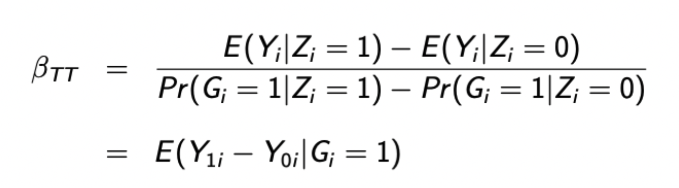
The above formula is true when there are no non-compliers (i.e. everyone who is assigned to treatment receives it). Otherwise this is the formula for the LATE (compliers) rather than the ATT (compliers and always takers)

Issues with external validity for RCTs

1. Extrapolation - impact on the studied group not being informative about other groups

2. Randomisation bias - Selection problem into the random sample so not representative of general population

3. General equilibrium effects - How does the RCT impact its results (i.e. the trial process may impact results in itself, rather than isolating the results of the treatment)

4. Hawthorne effect - people modify their behaviour because they know they’re being observed

5. John Henry effect - control group becomes aware they are a control, so put in extra effort to compensate for this perceived disadvantage.

Other problems with RCTs

• Expensive

• Difficult to recruit

• Not always usable (i.e. impact of monetary policy on growth)

• Need a sufficient population size to detect effects

• Problematic over long time periods

• Setting is often artificial without substantive theory

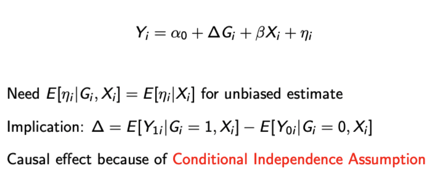
Formula for including observables in regression framework for treatment effects

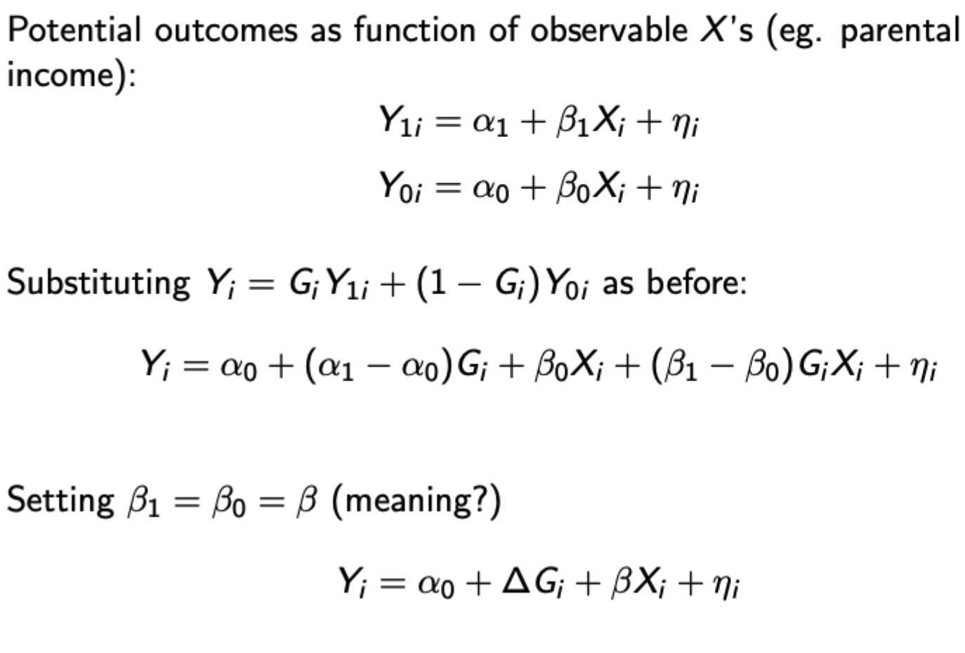
Setting beta(1) = beta(0) indicates that the effect of observables is the same with or without treatment

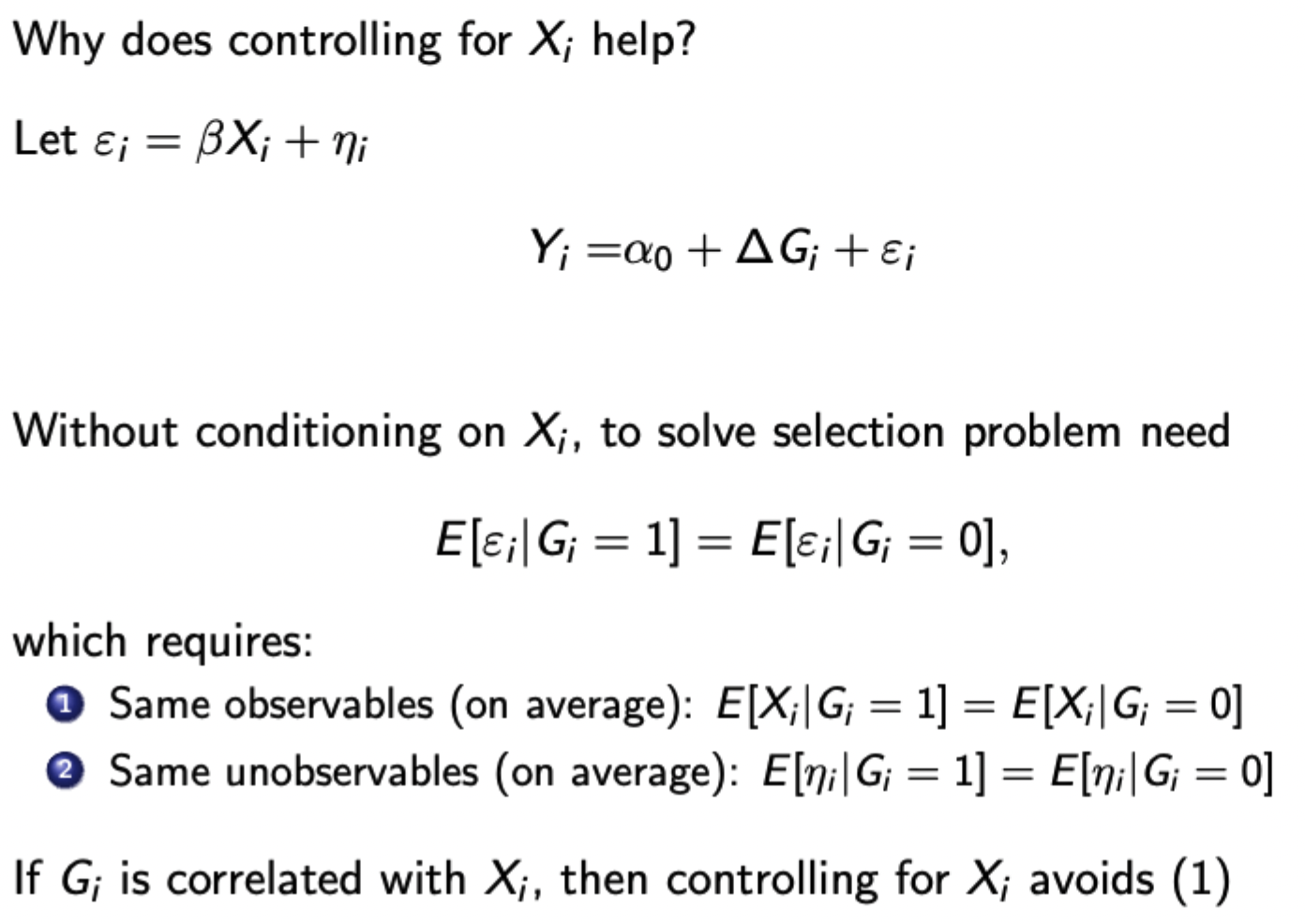
Why does controlling for observables reduce bias in estimating treatment effects

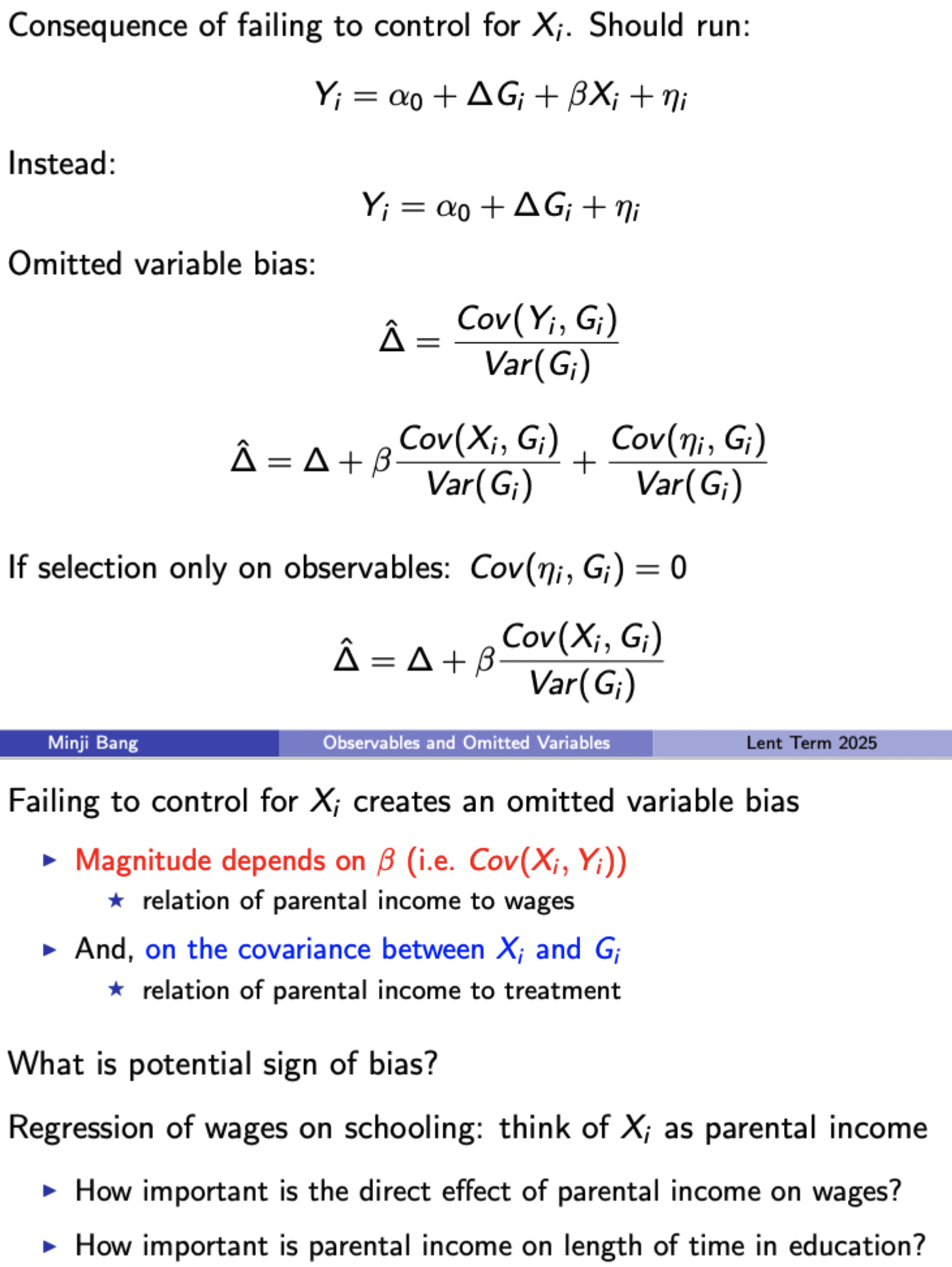
Consequences of failing to control for observables

Exclusion restriction

The instrument cannot have a direct effect on the dependent variable - i.e. should not belong in the regression when the endogenous variable is included

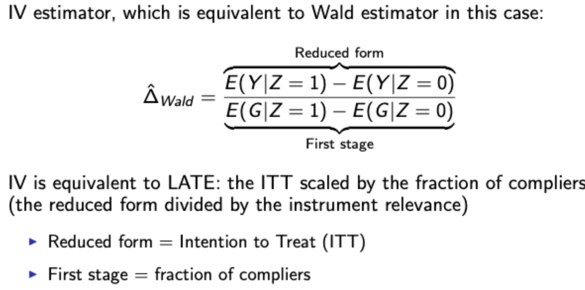
IV formula, interpretation wrt. 2SLS, and the modification to the Wald Estimator when treatment is binary

LATE - Local average treatment effect

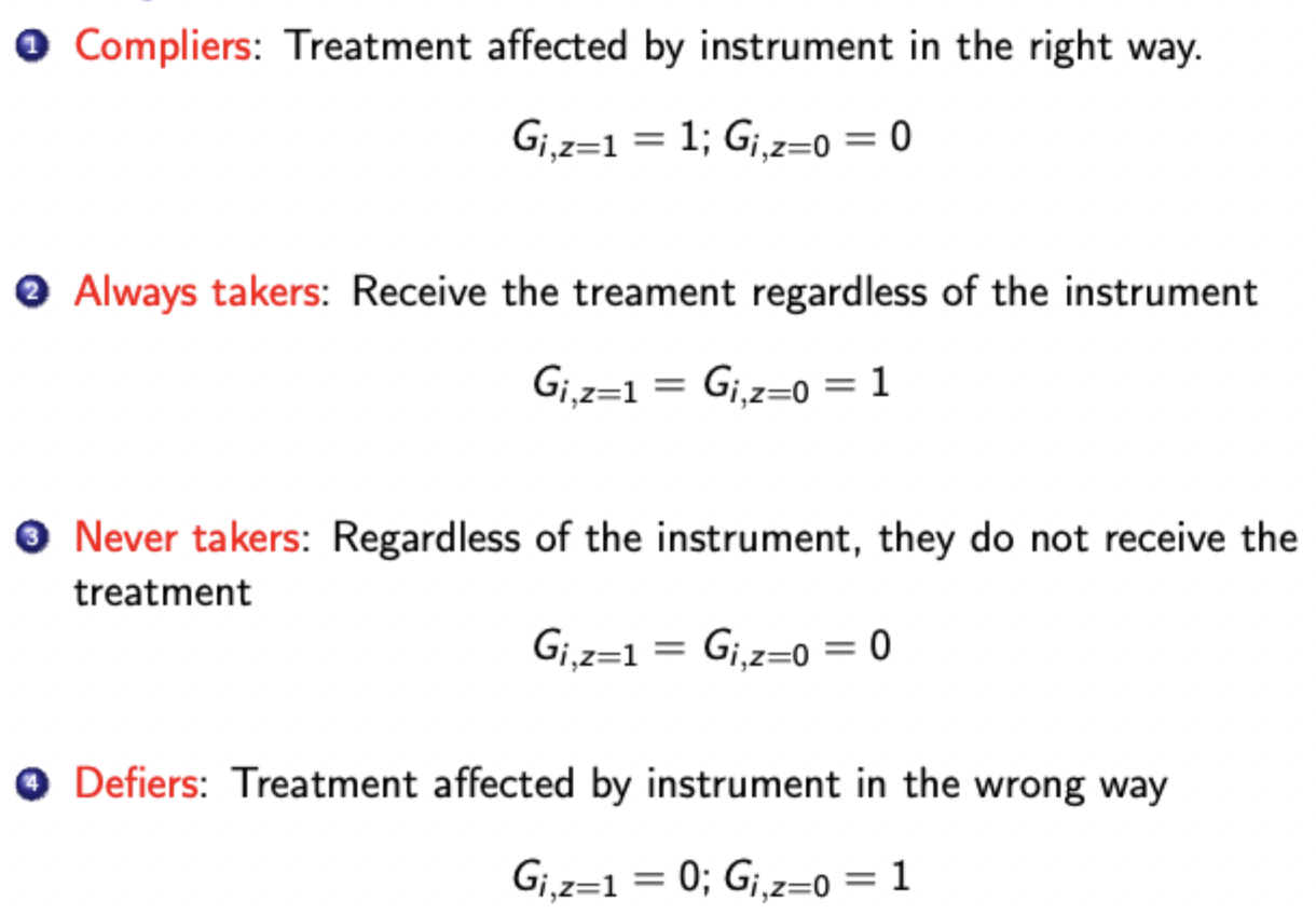
If only some individuals are affected by the instrument, teh IV is calculating the LATE, the ATE on those whose status has changed because of the instrument. Otherwise known as the ATE for for compliers (assuming that there are no defiers)

LATE not informative for always or never takers (those who will / won’t receive the treatment regardless of the IV)

Definitions - compliance / non-compliance

Wald estimator and ITT intuition

Using. the Wald estimator is equivalent to finding the LATE - the ITT scaled by the fraction of compliers

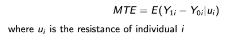
MTE - marginal treatment effect with continuous IV

The treatment effect for individuals who are on the margin between receiving treatment and not at different ‘resistance levels’ (unobserved factors pushing agents away from getting treated)

Used when the group of compliers are particularly different from the general population, indicating the LATE would not be of interest.

MTE implementation framework

Estimate propensity score P(Z) using continuous instrument (probability of treatment given instrumental value)

Estimate the relationship between Y and P(Z) via local polynomial regression (e.g. regress Y on linear and quadratic terms of P(Z)). This will give a reduced form polynomial.

Take derivative of the reduced form polynomial wrt. P(Z). Utilise the fact that at the margin, P(Z) (individual’s probability of treatment) = resistance, u (individual’s forces pushing them away from treatment), to evaluate the derivative at different values of u between 0 and 1.

MTE Interpretation

A downward slope between MTE and resistance suggests that individuals who choose to be treated (low resistance) are those who would expect to benefit most from it, whereas people who opt out (high resistance) would do so because they would expect the treatment not to help them. This is selection on gains / positive selection into treatment.

MTE can therefore be useful for policy targeting because it can show more accurately the returns to treatment from expanding out the treatment group in the presence of heterogeneous treatment effects. In the presence of selection on gains, policymakers may do well to limit the treatment to the group of compliers, since the effects on higher resistance individuals (i.e. never takers) are lower, so average effectiveness may fall if they are treated. This would indicate that the LATE overestimates the population ATE.

Integrating MTE

ATE: integrate MTE curve over all of u

ATT: integrate MTE curve only over low u

ATU (average treatment effect on the untreated): integrate only over high u

LATE: integrate over a specific part of u

Continuous IV isn’t necessary for MTE but is necessary to get the full range of P(Z) to estimate polynomial

Issues with MTE

P(Z) must have sufficient support (should be values pretty much over the whole unit interval)

Assumes instrument monotonicity (i.e. it affects everyone the same way)

Specification of each stage matters (i.e. specification for estimating propensity score, and specification for estimating reduced form polynomial between P(Z) and Y.

Fixed effects and DiD

FEs estimators deal with unobserved heterogeneity as a source of endogeneity that is fixed over time (or across individuals). Dealt with by using panel data and including individual (or time) - specific dummies or demeaning / first differencing the data to remove the individual FEs

DiD is a particular form of FEs that can be used with more aggregated data (doesn’t need to be a panel as it doesn’t have to track specific individuals through time, just an aggregate variable)

DiD process

Assuming treatment only occurs for i at period t, you difference across individuals to remove time dummies, then difference these difference to remove individual / group dummies, giving:

Assuming treatment occurs in periods after a certain point, you can group the time period into 2: period 0 (before / without treatment) and period 1: (after / with treatment). You can do the same with individuals: control group and treatment group. These simple 2×2 DiD’s can be seen as a form of FE estimator.

Parallel trends assumption and how it influences estimation DiD

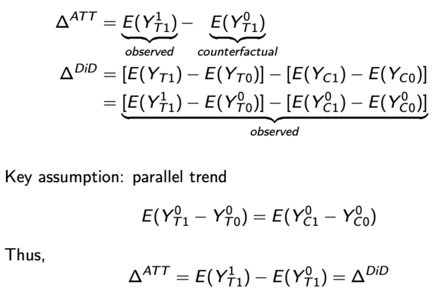
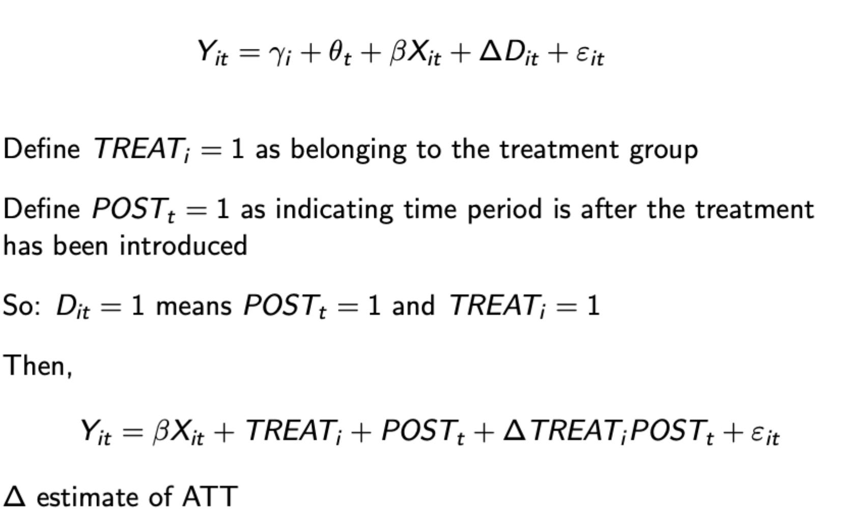
Regression representation of DiD

Remember group exogeneity assumption (those in the control group stay in the control group)

Why might an IV be needed for a FE estimator

FE estimator used when you have data on individuals over time

Differences are dealt with by differencing over time, assuming that treatment status varies with time (i.e. at some point people are treated)

However this throws away much of the individual variation, which may exacerbate measurement error if already there. Therefore, because of increased noise and potential endogeneity, a valid instrument is often needed.

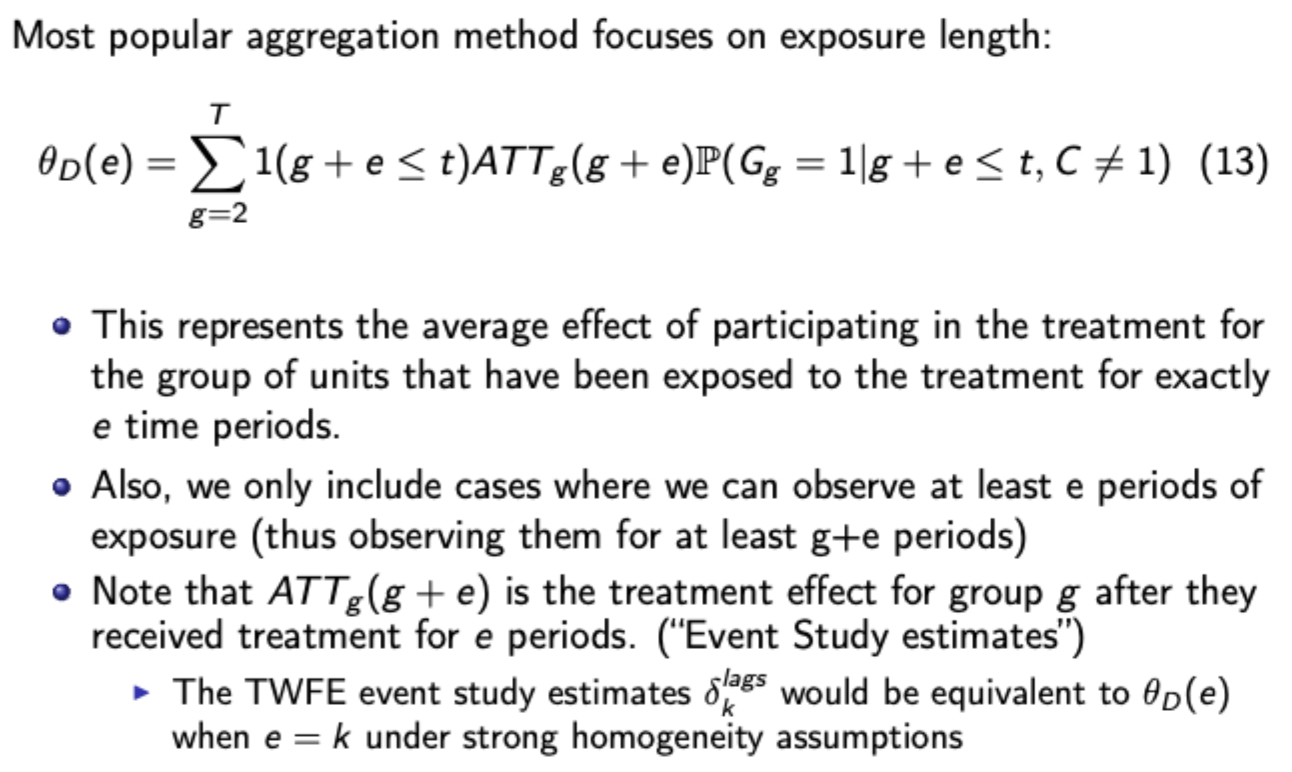
Formula for event study two way fixed effects (TWFE) spec

Where D^(k)_(it) is the indicator for unit i being k periods away from initial treatment at t

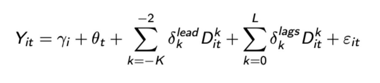
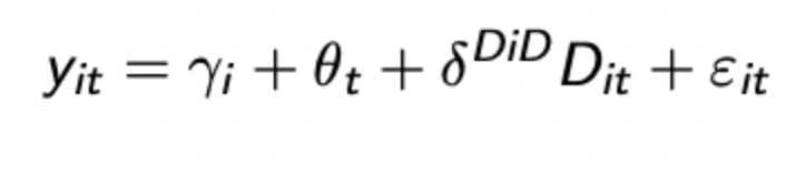
Once all coefficients estimated they can be combined into the below expression

Advantages of using traditional TWFE (i.e. regression DiD) even in staggered settings

• Provides estimates and SEs

• Easy to add additional units / periods

• Can include covariates / time trends etc.

Standard assumptions for event study designs

• Parallel trends: Evolution of untreated outcomes the same between treated + untreated groups

• No anticipation effects: no TEs before treatment occurs

• Treatment homogeneity across units

  • SUTVA: Stable unit treatment value assumption: no interference between units (treatment of one unit doesn’t affect other units’ outcomes)

Basic Issues of TWFE framework for event study design

The final DiD coefficient with staggered treatment timing is a weighted average of many treatment effects, with weights often negative and unintuitive

Additionally, as shown by Goodman-Bacon decomposition, some of the included TEs make no sense.

Goodman-Bacon Decomposition (GBD): Calculating the number of DiD estimates, and the core problem with some of them

In general, there are K timings groups for treatment, meaning that there are K² - K timings-only estimates (2×2 DiD estimates comparing an earlier vs later treated group), and then K 2×2 DiD estimates against untreated groups, giving a total of K² DiD estimates.

The issue is that some of them (comparing a late treatment with an early treatment after the earlier treatment) use already treated units as controls for the treated group in the late period. Control group already experiencing treatment effects so this is problematic.

Calculating weights for the TWFE estimator decomposed via GBD

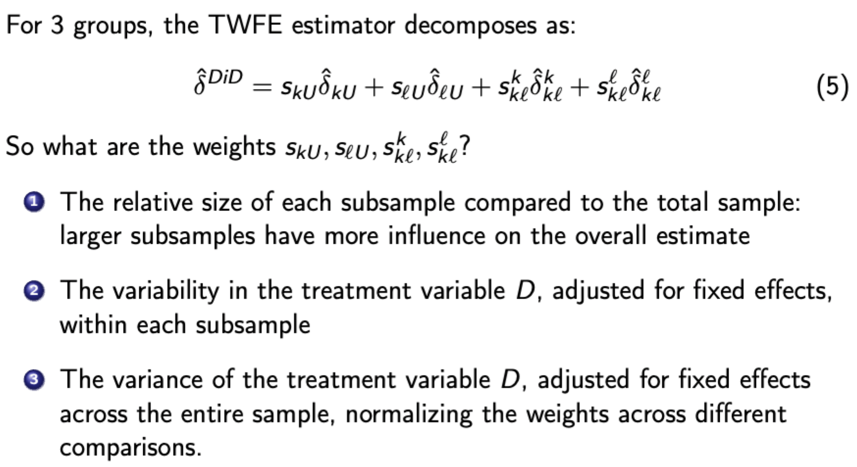
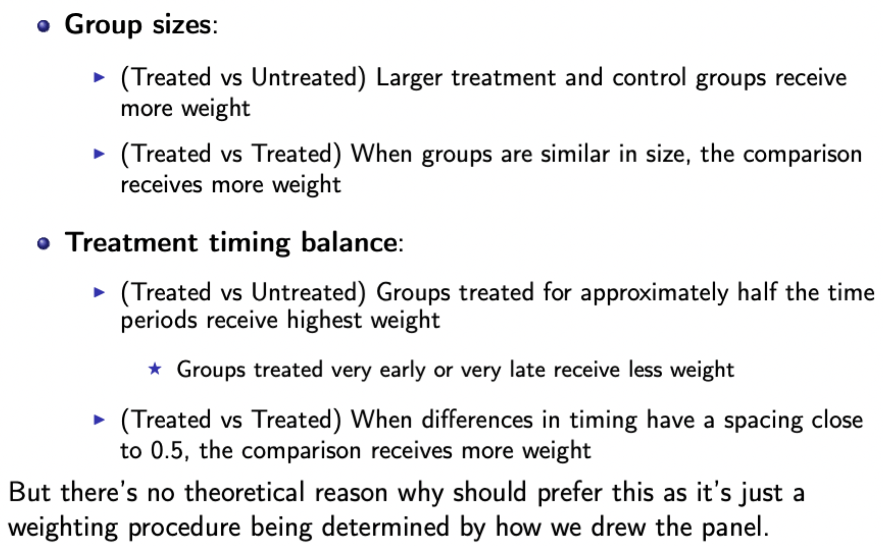
More balanced group sizes give a more precise DiD estimate

Variance matters, since you want more overlap between the groups, giving higher variance of D.

Key Insights of the GBD

Breaks down the TWFE estimator to help diagnose and understand potential biases.

The staggered DiD estimator from TWFE is the weighted average of all possible 2×2 DiD estimators, with already treated units acting as controls in some cases

Panel length can substantially change DiD estimates even when TEs don’t change

Groups treated closer to the middle of the panel receive higher weights

Some comparisons may receive negative weights, especially with heterogenous TEs

Identifying assumptions in potential outcomes framework for staggered DiD

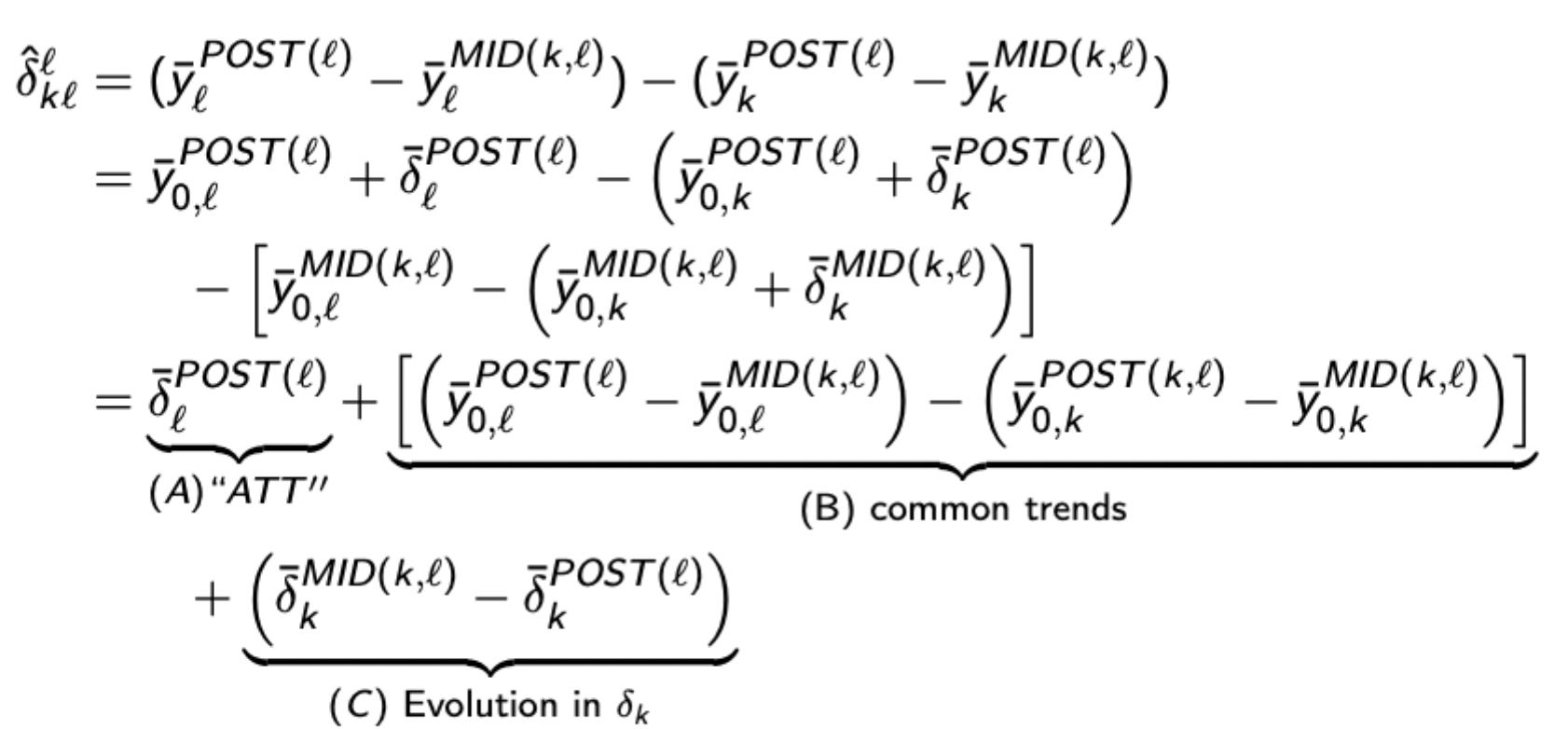
Identifying which key assumptions are violated by TWFE estimation of staggered DiD

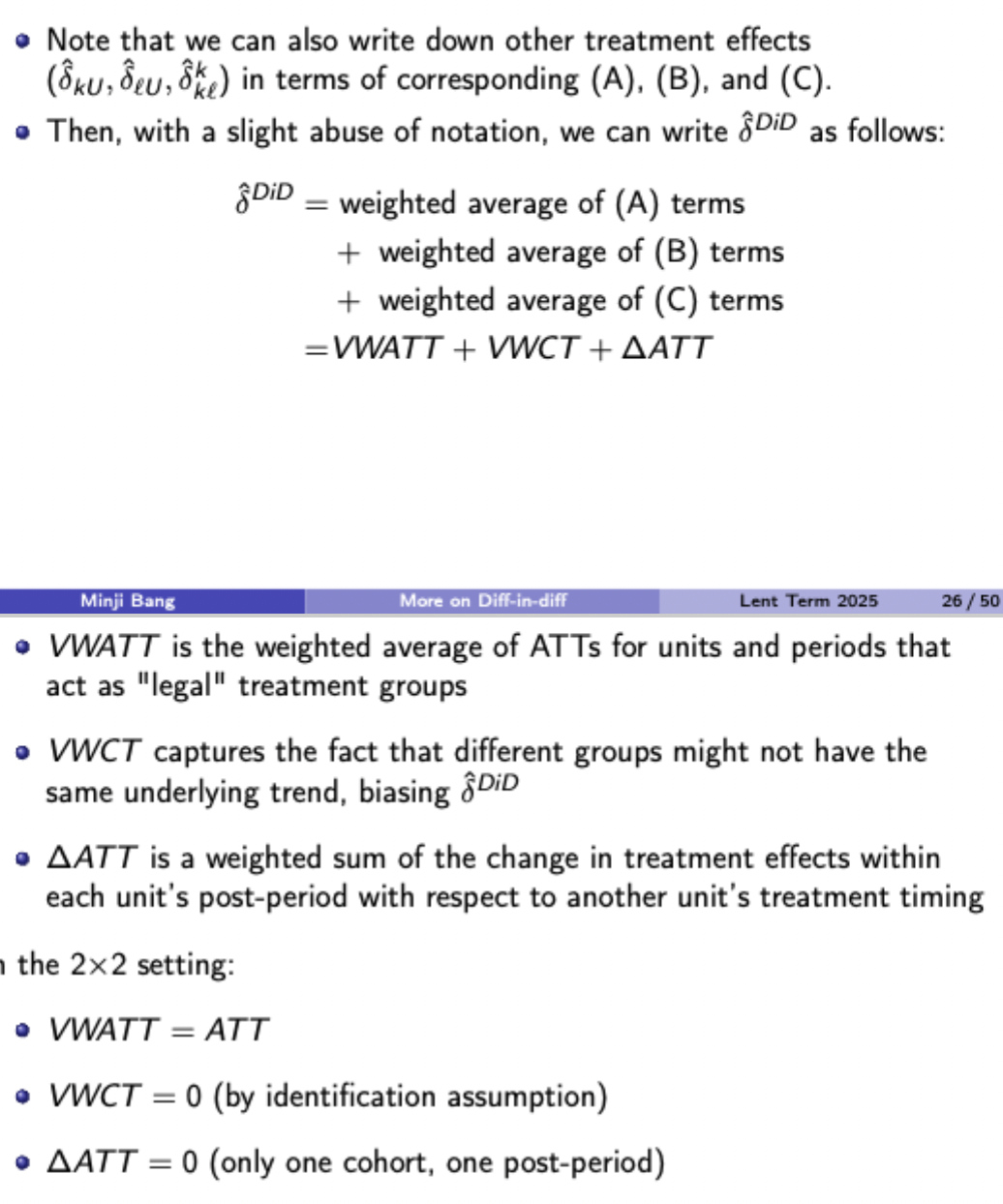
Delta ATT doesn’t = 0 when using treated k as a control for newly treated l

VWCT doesn’t = 0 when comparing l vs k with different underlying trends

Key idea of Callaway and Sant’Anna’s solution to staggered DiD problem

Decompose the TWFE DiD into several 2×2 DiD comparisons, then eliminate all ‘forbidden comparisons’ (treated units as controls) and focus on 2×2 comparisons to capture heterogeneity due to staggered timing

Callaway and Sant’Anna: Key Assumptions

• No treatment anticipation

• Bounded propensity score (never >= 1), ensuring positive probability of receiving treatment and avoids perfect prediction by covariates

• Conditional parallel trends

  • Conditional on covariates, the expected outcome trend without treatment is the same for treatment and control groups

C&SA estimator for key parameter

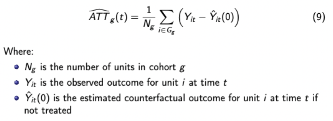
Advantages of group-time ATTs

• Allows for TE heterogeneity across groups

• Avoids using already treated units as controls

• Controls can be never treated or not yet treated units

• Flexible conditioning on covariates

• Natural connection to event studies

• Can be aggregated in various ways to answer different policy questions

Ways of combining group-time ATTs for C&SA method

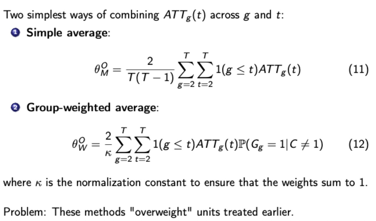
Use of exposure length for dynamic treatment effects

C&SA method: pros and cons

Pros:

• Avoids bias from forbidden comparisons

• Allows for heterogeneous treatment effects

• Flexible conditioning on covariates

• Multiple aggregation options

Cons

• Computational complexity increases with number of groups

• Many parameters to estimate and interpret

• Requires more data than traditional DiD

• Utilises bootstrap procedures (computationally intensive)

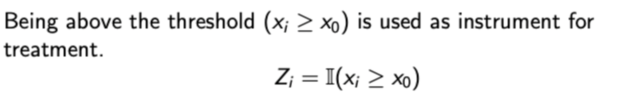
Regression discontinuity formula

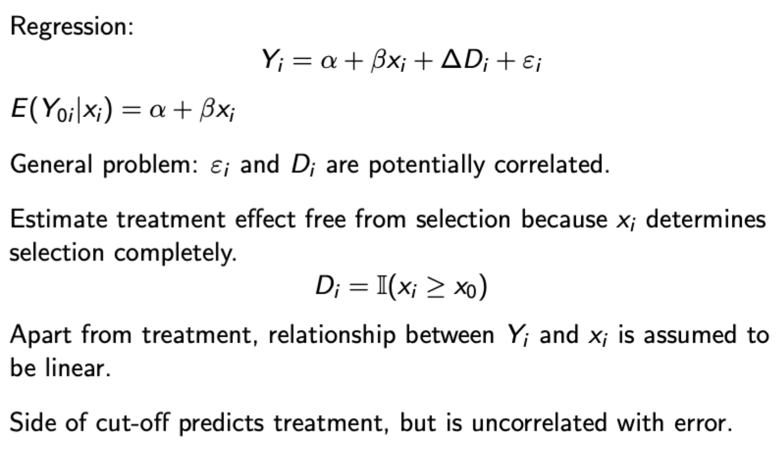
Selection is a deterministic function of the running variable x(i), and close to the threshold the treatment and control groups are effectively the same, except one group receives treatment.

This method doesn’t rely as much on fitting the trend well

Difference between precise, imprecise and complete control over running variable in the presence of a cutoff

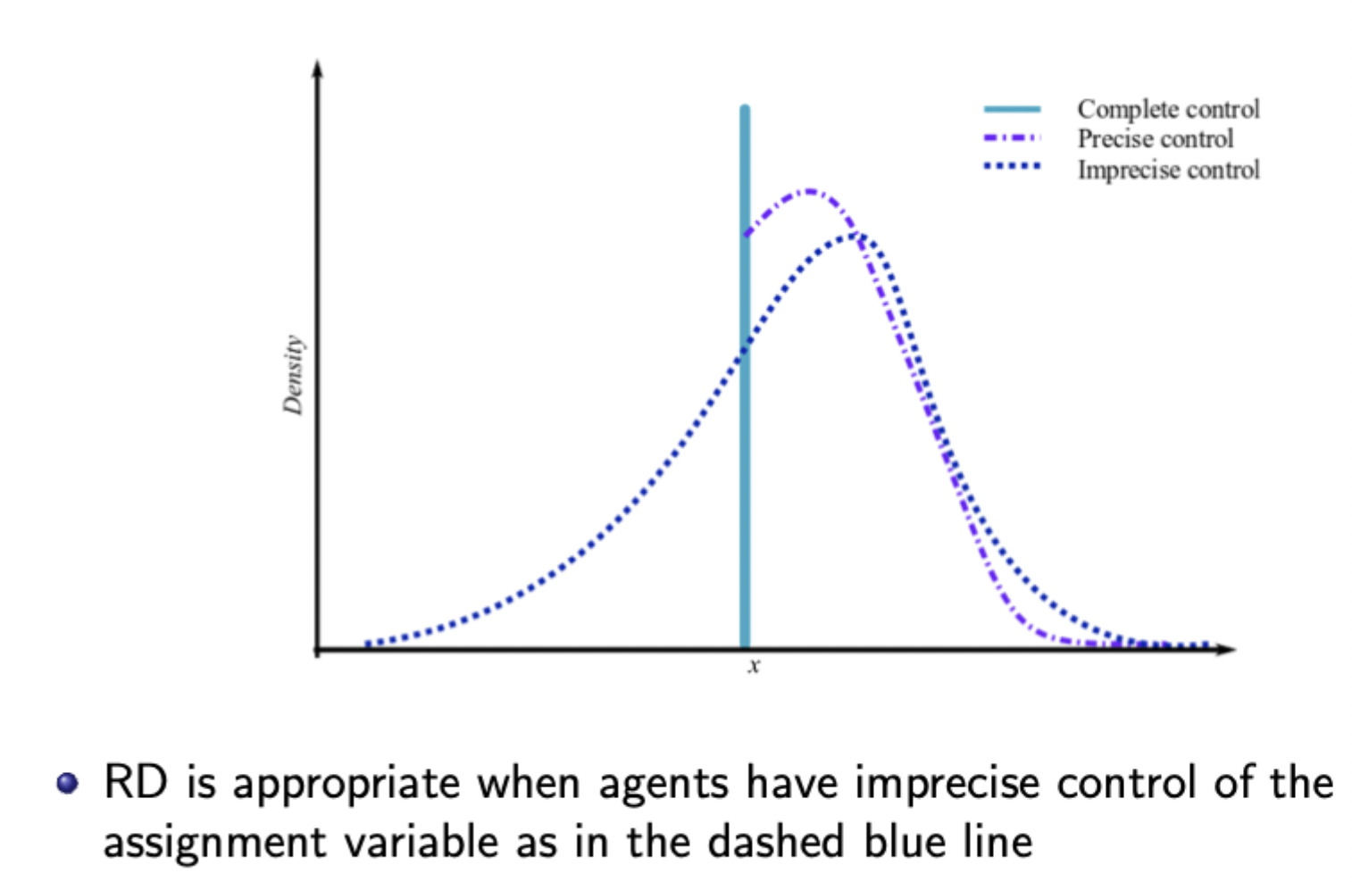
When control is imprecise, treatment is ‘as good 'as’ randomly assigned around the cutoff (i.e. there will still be observations that fall either side of the cutoff with very similar covariates)

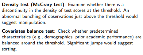
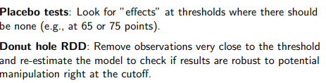
Testing for manipulation of the running variable

1. Balanced covariates: no difference in predetermined covariates either side of the cutoff, and can also check that relevant covariates evolve smoothly round the cutoff

2. Continuous density: density of x should be continuous at the cutoff - with manipulation there is an abnormal spike around the cutoff area.

Basic steps to running RDD

1. Graph the raw data (treatment and outcome graphs and then density of the assignment variable.

2. Estimate regressions to provide estimates of treatment effects (run separate regressions either side of cutoff or run a pooled regression

3. Test validity (no manipulation assumption, McCreary density test to show continuous density, also vary the bandwidth and order of polynomial to test robustness

4. Including covariates (when RD is valid, these should be orthogonal to D conditional on X and similar on both sides of the cutoff)

Parametric vs nonparametric methods for fitting functions of the assignment variable either side of the cutoff

Parametric: polynomial models (increase powers in X starting with linear regression) - may be erratic around cutoff

Non-parametric: estimate linear regression in cutoff region using smaller and smaller bandwidths (closer in spirit to the RD concept - focus on the cutoff)

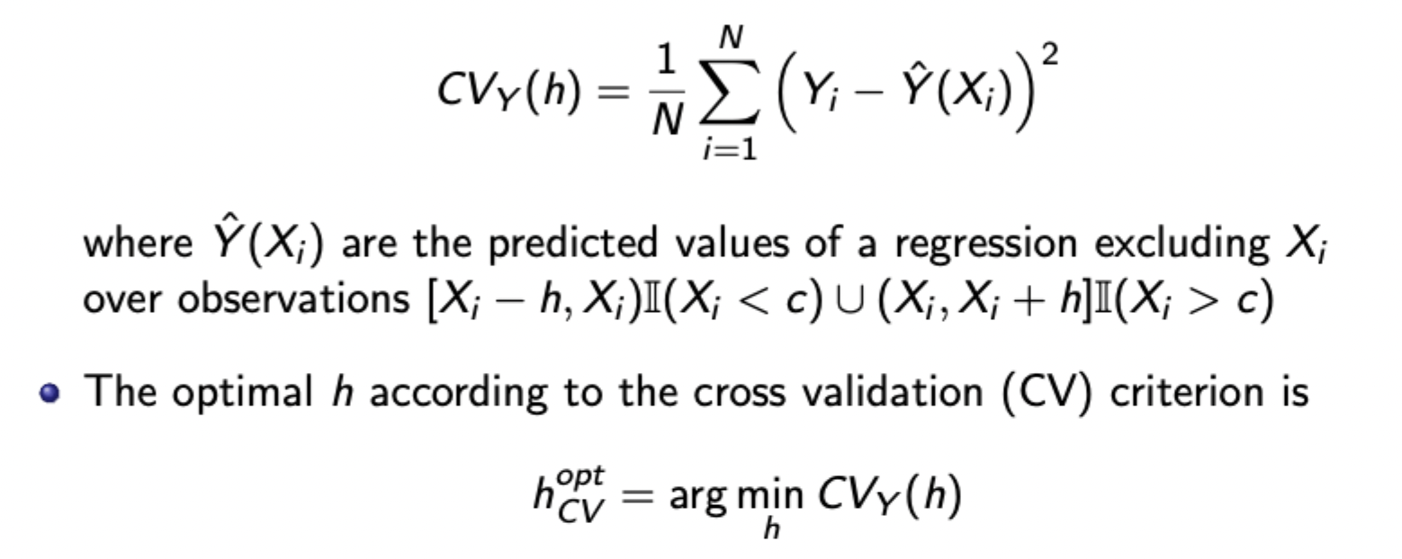
Choosing optimal bandwidth for nonparametric RDD - Cross validation criterion

Tradeoff loss of efficiency from small h with increase in bias (if the underlying conditional expectation is nonlinear) with large h

Choose to minimise CV criterion:

Fuzzy RDD

Treatment probability changes discontinuously at the cutoff, but not necessarily from 0 to 1. Non-perfect compliance in action (some individuals who should receive treatment do not)

Therefore, think of fuzzy RDD as an IV estimator of the LATE (as done before). The instrument is relevant and exogenous, shown below:

Requires monotonicity assumption (cross threshold cannot reduce probability of treatment) and no defiers (as defiers cancel estimated TEs)

Key advantage of GMM

• Allows for over identification from moment conditions

• Optimally combines info from all moment conditions

• Provides efficiency gains when the weighting matrix is optimal

• Robust to error heteroskedasticity

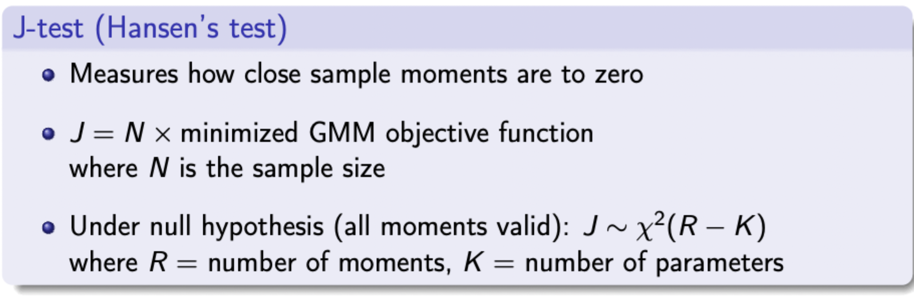
Testing overidentifying restrictions

GMM Implementation

1. Define problem + parameters

2. Use economic theory to identify at least K moment conditions

3. Collect data and use sample moments

4. Choose initial weighting matrix (often identity matrix)

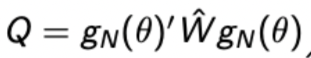
5. Estimate parameters that minimise quadratic form expression

6. Update weighting matrix using first step estimates

7. Minimise again with updated weighting matrix

8. Calculate SEs and test statistics

GMM objective function

SEs for GMM

When to use GMM

When full distributional assumptions (i.e. for MLE) are questionable

For non-standard estimation problems (e.g. dynamic panels)

MLE more robust, GMM more efficient

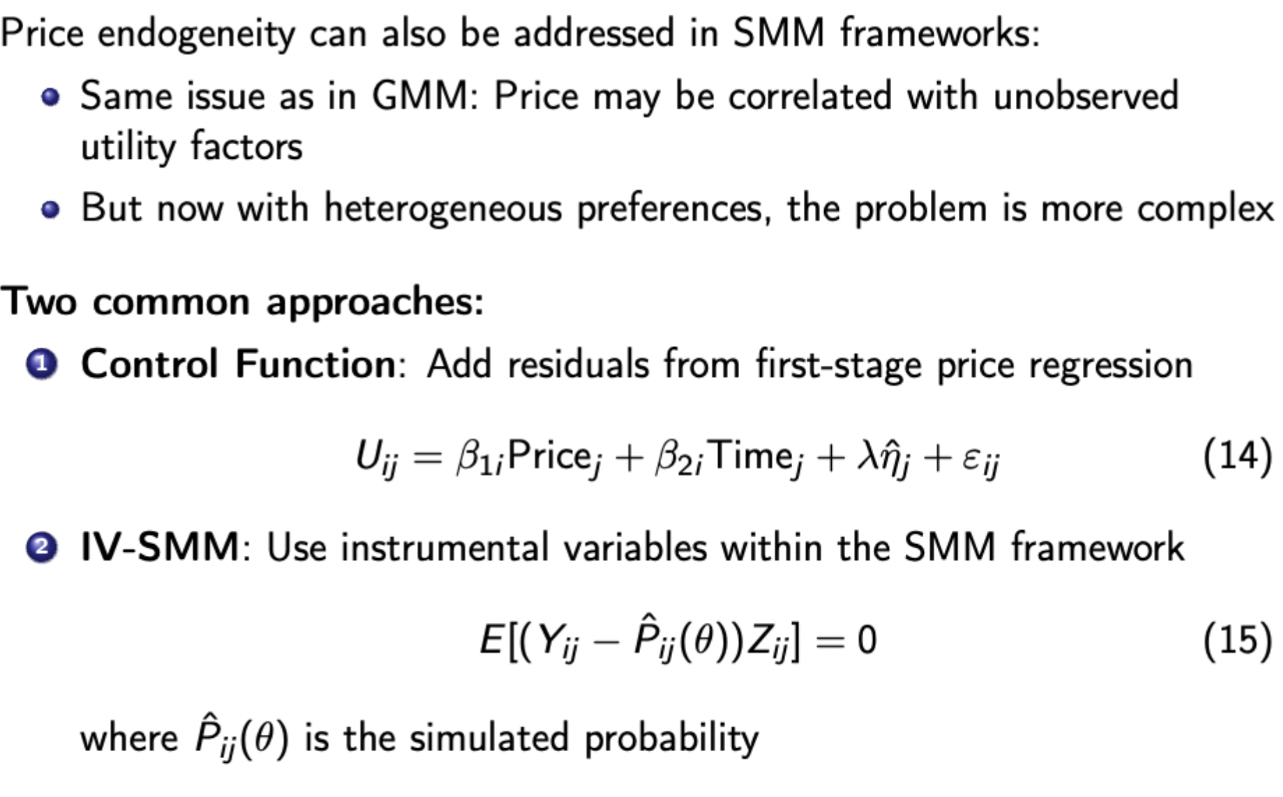
SMM example for discrete choice model with preference heterogeneity

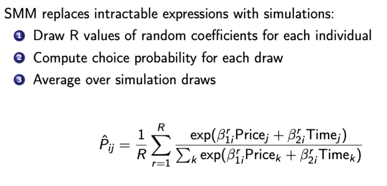
From random coefficients model

Tradeoffs with SMM

Larger R means more accurate approximation but computation cost is linearly increasing in R

In practice, start with small R and increase as you get closer to the optimum, then complete final estimation with large R.

Dealing with endogeneity in SMM frameworks

SMM estimation process

1. For given parameters, simulate choice probabilities

2. Compute moment conditions

3. Minimise objective function using simulated probabilities

Bootstrap method

Resample dataset with replacement, the re-estimate the model for each bootstrap sample. Look at the distribution of estimates across samples.

Why are bootstrap SEs useful for SMM

They are conceptually simple unlike analytical SEs which are very complicated for SMM (simulation has additional noise, derivatives are complex, need to account for simulation error etc.)

Methods to find bootstrap confidence intervals

1. Percentile method: use 2.5th and 97.5th percentile of boostrap distribution

2. Bias-corrected method: adjusts for potential bias in distribution, more accurate but more complex

Specification testing in SMM (i.e. over-identifying test to see if an instrument is valid)

Same principals as in Hansen’s test (j-test) for GMM.

1. Same asymptotic dist., but now with additional noise from simulation and need to account for simulation error. Critical values also depend on the number of simulation draws R.

2. The test statistic for SMM converges to that of GMM as R gets large. Therefore as a rule of thumb use large R for specification testing (much larger than parameter estimation)

Why might an IV estimator be larger or smaller than an OLS estimator

1. OLS is biased (measurement error, selection bias, OVB, etc.)

2. IV is biased (failure of exclusion restriction - exacerbated by weak instruments) (also remember DI case - OLS used when people don’t need to apply, whereas IV can only be used on applicants, so the samples are different and likely lead to a sample selection bias for the IV estimator)

3. Heterogeneity - IV and OLS are now estimating different things - OLS estimates ATT whereas IV estimates LATE. If there is treatment heterogeneity then the LATE estimate will be different to that of the ATT.

Relationship between the different treatment effect estimators

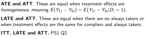
ITT, LATE, and ATT are the same when assignment to treatment is a perfect predictor of when an individual receives treatment (i.e. no always takers, no never takers, and no defiers)

Issues to consider when applying DiD

Common time trend

Potential non-linear effects

Spill over effects (i.e. moving from treatment group to untreated group after the treatment)

External validity

Implementing fuzzy RDD (test score example)

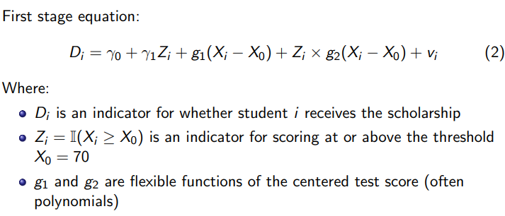
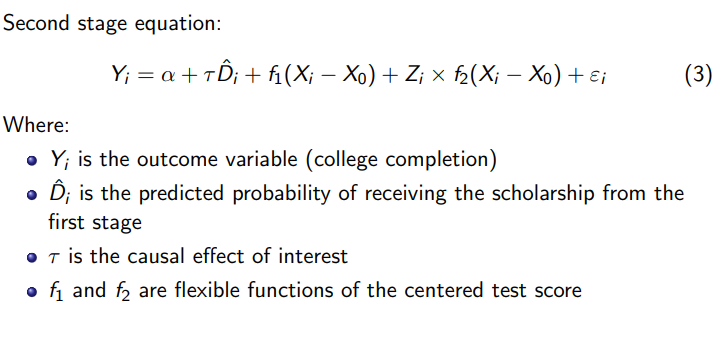
This is 2SLS. You include all other regressors including the ‘endogenous’ one in the first stage, estimated via different parameters. Also include interactions to show the effects of the test score around the cut off, and the additional effects of this due to assignment to treatment.

Summary of tests for manipulation of running variable around the cut off in RDD

Using parametric vs non-parametric methods when implementing normal / fuzzy RDD

Parametric (i.e. polynomial)

• Advantages: Uses all data points which potentially increases precision, can capture global patterns in the data

• Disadvantages: Potential misspecification of functional form, may be influenced by observations very far from the threshold, and potentially sensitive to overspecification

Non-parametric (i.e. LLR):

• Advantages: Focuses on observations near the cut-off where identification is strongest, less sensitive to functional form misspecification, better approximation of the true relationship near the cut-off

• Disadvantages: Requires choosing a bandwidth, might use fewer observations which reduces precision, more complex to implement.

Key factors influencing the decision:

• Sample size: With larger samples, non-parametric approaches become more feasible

• Data pattern: if relationship between test scores and outcomes appears highly non-linear, parametric models may be less appropriate, since it may be less likely that you correctly specify the functional form, leading to bias.

• Distance from threshold: if we’re primarily interested in effects very close to the threshold, local approaches are preferable

• Bandwidth selection: availability of formal methods for optimal bandwidth selection makes non-parametric approaches more credible.

• Robustness checks: Best practice would be to implement both approaches and check sensitivity of results.