Data Structures and Algorithms

Terms and concepts for Data Structures and Algorithms

What is an algorithm?

A method or set of rules that must be followed when performing problem solving operations. As a result, an algorithm is a collection of rules or instructions that govern how a work is to be conducted step-by-step to achieve the desired results

Finiteness

An algorithm must always have a finite number of steps before it ends. When the operation is finished, it must have a defined endpoint or output and not enter an endless loop.

Definiteness

An algorithm needs to have exact definitions for each step. Clear and straightforward directions ensure that every step is understood and can be taken easily.

Input

An algorithm requires one or more inputs. The values that are first supplied to the algorithm before its processing are known as inputs. These inputs come from a predetermined range of acceptable values.

Output

One or more outputs must be produced by an algorithm. The output is the outcome of the algorithm after every step has been completed. The relationship between the input and the result should be clear.

Effectiveness

An algorithm's stages must be sufficiently straightforward to be carried out in a finite time utilizing fundamental operations. With the resources at hand, every operation in the algorithm should be doable and practicable.

Generality

Rather than being limited to a single particular case, an algorithm should be able to solve a group of issues. It should offer a generic fix that manages a variety of inputs inside a predetermined range or domain.

Modularity

This feature was perfectly designed for the algorithm if you are given a problem and break it down into small-small modules or small-small steps, which is a basic definition of an algorithm.

Correctness

An algorithm's correctness is defined as when the given inputs produce the desired output, indicating that the algorithm was designed correctly. An algorithm's analysis has been completed correctly

Maintainability

It means that the algorithm should be designed in a straightforward, structured way so that when you redefine the algorithm, no significant changes are made to the algorithm.

Functionality

It takes into account various logical steps to solve a real-world problem.

Robustness

Robustness refers to an algorithm's ability to define your problem clearly.

User-friendly

If the algorithm is difficult to understand, the designer will not explain it to the programmer

Simplicity

If an algorithm is simple, it is simple to understand

Extensibility

Your algorithm should be extensible if another algorithm designer or programmer wants to use it.

Brute Force Algorithm

A straightforward approach that exhaustively tries all possible solutions, suitable for small problem instances but may become impractical for larger ones due to its high time complexity.

Recursive Algorithm

A method that breaks a problem into smaller, similar subproblems and repeatedly applies itself to solve them until reaching a base case, making it effective for tasks with recursive structures

Encryption Algorithm

Utilized to transform data into a secure, unreadable form using cryptographic techniques, ensuring confidentiality and privacy in digital communications and transactions.

Backtracking Algorithm

A trial-and-error technique used to explore potential solutions by undoing choices when they lead to an incorrect outcome, commonly employed in puzzles and optimization problems

Searching Algorithm

Designed to find a specific target within a dataset, enabling efficient retrieval of information from sorted or unsorted collections

e.g. to find numbers and sets, to find the shortest distance to get to a location

Sorting Algorithm

Aimed at arranging elements in a specific order, like numerical or alphabetical, to enhance data organization and retrieval.

Hashing Algorithm

Converts data into a fixed-size hash value, enabling rapid data access and retrieval in hash tables, commonly used in databases and password storage.

Divide and Conquer Algorithm

Breaks a complex problem into smaller subproblems, solves them independently, and then combines their solutions to address the original problem effectively.

Greedy Algorithm

Makes locally optimal choices at each step in the hope of finding a global optimum, useful for optimization problems but may not always lead to the best solution.

Dynamic Programming Algorithm

Stores and reuses intermediate results to avoid redundant computations, enhancing the efficiency of solving complex problems.

Randomized Algorithm

Utilizes randomness in its steps to achieve a solution, often used in situations where an approximate or probabilistic answer suffices.

Recursive algorithms

Recursive algorithms are a fundamental concept in computer science, particularly in the study of data structures and algorithms. A recursive algorithm is one that solves a problem by breaking it down into smaller instances of the same problem, which it then solves in the same way. This process continues until the problem is reduced to a base case, which is solved directly without further recursion.

Key Concepts of Recursive Algorithms - Base Case

This is the condition under which the recursion stops. It represents the simplest instance of the problem, which can be solved directly without further recursion.

Key Concepts of Recursive Algorithms - Recursive Case

This is the part of the algorithm that breaks the problem down into smaller instances of the same problem and then calls the algorithm recursively on these smaller instances.

Key Concepts of Recursive Algorithms - Stack

Each recursive call is placed on the system call stack. When the base case is reached, the stack begins to unwind as each instance of the function returns its result

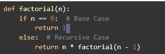
Factorial Calculation

The factorial of a number n (denoted as n!) is a classic example of a recursive algorithm. The factorial is defined as:

• O! = 1 (Base Case)

• N! = n * (n-1)! For n > O (Recursive Case)

How It Works:

• Base Case: When n is 0, the function returns 1.

Recursive Case: For any other value of n, the function calls itself with n−1 and multiplies the result by n.

Simplicity

Recursive solutions are often more elegant and easier to understand than their iterative counterparts

Direct Translation

Some problems are naturally recursive, like tree traversals, making recursion the most straightforward approach

Performance

Recursive algorithms can be less efficient due to the overhead of multiple function calls and potential stack overflow issues for deep recursion

Memory Usage

Recursion can consume more memory because each function call adds a new frame to the call stack

When to Use Recursion

• When a problem can naturally be divided into similar sub-problems (e.g., tree traversal, searching algorithms like binary search).

• When the recursive solution is significantly simpler or more intuitive than an iterative one.

Binary Search

Concept:

• Binary search is much more efficient than linear search but requires the array or list to be sorted.

• It works by repeatedly dividing the search interval in half. If the target value is less than the middle element, the search continues in the left half, otherwise in the right half.

Algorithm:

1. Start with two pointers, one at the beginning (low) and one at the end (high) of the sorted array.

2. Find the middle element of the current interval.

3. Compare the middle element with the target:

   • If they match, return the index of the middle element.

   • If the target is less than the middle element, repeat the search on the left half.

   • If the target is greater, repeat the search on the right half.

4. If the interval becomes invalid (low > high), return a "not found" indication.

Time Complexity: O(log⁡ n), where n is the number of elements in the array. This logarithmic time complexity makes binary search significantly faster than linear search for large datasets.

When to Use:

• When the array or list is sorted.

• When the array is large and efficiency is crucial.

Linear Search

Concept:

• Linear search is the simplest search algorithm.

• It works by sequentially checking each element of the array or list until the target element is found or the end of the collection is reached.

Algorithm:

1. Start from the first element of the array.

2. Compare the current element with the target element.

3. If they match, return the index of the element.

4. If they don't match, move to the next element and repeat the process.

5. If the target element is not found by the end of the array, return a "not found" indication.

Time Complexity: O(n), where n is the number of elements in the array. This is because in the worst case, the algorithm may need to check every element in the array.

When to Use:

• When the array or list is small.

• When the array is unsorted.

• When simplicity is more important than performance.

• Linear Search Worst, Average and Best

  • Best Case: O(1) — The target element is the first element.

  • Average Case: O(n) — The target element is somewhere in the middle or not in the array.

  • Worst Case: O(n) — The target element is the last element or not present.

Record or Struct

a data structure that stores subitems

Search Algorithms

Broadly categorized into linear, binary, and graph traversal algorithms

Binary Search

The primary method for searching an item in a sorted array, which repeatedly divides the search interval in half until the target value is found or the interval is empty.

How Binary Search Works:

• It starts by comparing the target value with the middle element of the sorted array. 

• If the target value matches the middle element, the search is successful, and the index of the middle element is returned. 

• If the target value is less than the middle element, the search continues in the left half of the array. 

• If the target value is greater than the middle element, the search continues in the right half of the array. 

• This process is repeated until the target value is found or the search interval becomes empty. 

Interpolation Search

• Concept: Similar to binary search but works on uniformly distributed data. It estimates the position of the target element based on the value.

• Time Complexity: O(log ⁡log ⁡n) in the best case, O(n) in the worst case.

• Use Case: Effective when the data is uniformly distributed.

• Interpolation Search Worst, Average and Best

  • Best Case: O(1) — The target element is exactly where the interpolation suggests.

  • Average Case: O(log ⁡log⁡ n) — Uniformly distributed data.

  • Worst Case: O(n) — Highly skewed data distribution or worst interpolation.

Depth-First Search (DFS) and Breadth-First Search (BFS)

• Concept: Used primarily in graph and tree data structures. DFS explores as far as possible along one branch before backtracking, while BFS explores all neighbors at the present depth before moving on to nodes at the next depth level.

• Time Complexity: O(V+E), where V is the number of vertices and E is the number of edges.

• Use Case: Useful for searching nodes in graphs and trees.

• Depth-First Search (DFS) Worst, Average and Best

  • Best Case: O(1) — The target node is found immediately.

  • Average Case: O(V+E)— Typically when all nodes and edges must be explored.

  • Worst Case: O(V+E) — The target node is the last one discovered.

• Breadth-First Search (BFS) Worst, Average and Best

  • Best Case: O(1) — The target node is the root or the first node checked.

  • Average Case: O(V+E) — All nodes and edges need to be explored.

  • Worst Case: O(V+E) — The target node is the last one explored.

Time Complexity Analysis

describes how its execution time grows as the input size increases, often expressed using Big O notation, which focuses on the worst-case scenario

Logarithmic (as in "Logarithmic Time" or O(log n))

A logarithmic operation reduces the problem size by a consistent fraction each time—usually by half.

📌 In Big O terms:
An algorithm with O(log n) complexity takes fewer steps as the input size increases, because it cuts the input down rapidly.

🔍 Example:
Binary Search
If you have a sorted list of 1,000 items and want to find a specific one:

• First check the middle item.

• If it's too high or too low, discard half the list.

• Repeat until you find it.

Each time, the list gets cut in half:
1,000 → 500 → 250 → 125 → ...

So the number of steps grows logarithmically with the size of the list.

Array

An array is a data structure that stores a list of elements in a specific order in memory. Each element is accessible by its index (position number).

Dominant Term

In Big O notation, the dominant term is the one that grows fastest as the input gets larger. It determines how the performance of the algorithm scales.

📌 We ignore smaller terms and constants because they have less impact as the input grows.

🔍 Example:

def example(n):

return 3*n + 100Constant (as in "Constant Time" or O(1))

Even though 100 is added and 3 multiplies n, the n is the dominant term, so we write the complexity as O(n).

Constant (as in "Constant Time" or O(1))

A constant is a fixed value that does not change with the input size.

📌 In Big O, O(1) means the operation always takes the same amount of time, no matter how big the input is.

def print_first_item(arr):

print(arr[0])

Even if arr has 1 or 1 million items, accessing the first one is always constant time – O(1).

Also in expressions like O(n² + 2n + 7), the 7 is a constant, and in Big O, we drop it when analyzing performance.

Time Complexity

The Amount of time required to complete an algorithm’s execution

Big O Notation is used to represent an algorithm’s time complexity

Calculated primarily by counting the number of steps required to complete the execution

Space Complexity

The amount of space (RAM usage) an algorithm requires to solve a problem and produce an output

Expressed in Big O Notation

Comparison: Array & Linked List (Array)

• ordered and indexed collection of elements

• fixes-size (python)

• stored in contiguous memory locations

• used when we require random access to elements; when insertion & deletion are infrequent O(n)

Comparison: Array & Linked List (Linked List)

• linear data structure consisting of nodes and pointers

• used when the number of elements is not known in advance

• used in cases when faster insertion and deletion are required O(1)

Sorting Algorithms

Sorting algorithms organize data in a particular order (usually ascending or descending). This makes searching and other operations more efficient.

Bubble Sort

• Use Case: Simple but inefficient for large datasets. Best used for educational purposes or small lists.

• Distinct Characteristics:

• Repeatedly swaps adjacent elements if they are in the wrong order.

• Simple, but inefficient for large datasets.

• “Bubbles” the largest element to the end of the list.

• Bubble Sort Worst, Average and Best

  • Best Case: O(n) — The array is already sorted (with an optimized version that stops early).

  • Average Case: O(n²) — Average case with random elements.

  • Worst Case: O(n²) — The array is sorted in reverse order.

• Bubble: Look for something that swaps so the result can “bubble” to the top. (Swap, Exchange)

Selection Sort

• Use Case: Inefficient for large lists, but useful when memory writes are more expensive than comparisons.

• Distinct Characteristics:

• Finds the minimum element and swaps it with the first unsorted element.

• Reduces the problem size by one in each iteration.

• Always performs O(n²) comparisons, regardless of input.

• Selection Sort Worst, Average and Best

  • Best Case: O(n²) — Selection sort does not improve with better input, always O(n²).

  • Average Case: O(n²) — Average case with random elements.

  • Worst Case: O(n²) — Selection sort is insensitive to input order.

• Selection: Look for code that repeatedly finds the minimum (or maximum) element and moves it to the beginning (or end) of the list. (Select minimum, Swap with start)

Insertion Sort

• Use Case: Good for small or nearly sorted lists.

• Distinct Characteristics:

• Builds a sorted list one element at a time.

• Efficient for small or nearly sorted datasets.

• Shifts elements to make space for the current element.

• Insertion Sort Worst, Average and Best

  • Best Case: O(n) — The array is already sorted.

  • Average Case: O(n²) — Average case with random elements.

  • Worst Case: O(n²) — The array is sorted in reverse order.

• Insertion: Look for code that builds a sorted portion of the list one element at a time by inserting each new element into its correct position within the already-sorted part. (Insert, Shift Element)

Merge Sort

• Use Case: Efficient and stable; good for large datasets.

• Distinct Characteristics:

• Divides the list into halves, sorts each half, and then merges them.

• Stable and efficient for large datasets.

• Requires additional space for merging.

• Merge Sort Worst, Average and Best

  • Best Case: O(n log⁡ n) — Merge sort’s time complexity is the same in all cases.

  • Average Case: O(n log⁡ n).

  • Worst Case: O(n log⁡ n).

• Merge: Look for something that continually splits a list in half. (Merge, Split)

Quicksort

• Use Case: Often faster in practice than merge sort but less stable.

• Distinct Characteristics:

• Selects a “pivot” element and partitions the array around it.

• Recursively sorts the partitions.

• Efficient, but can degrade to O(n²) if poor pivot selection occurs.

• Quicksort Worst, Average and Best

  • Best Case: O(n log⁡ n) — The pivot splits the array into two nearly equal halves.

  • Average Case: O(n log⁡ n) — Average case with random pivots.

  • Worst Case: O(n²) — The pivot is always the smallest or largest element, leading to unbalanced partitions.

• Quicksort: Look for the keywords “pivot” and/or “split”. (Pivot, Split)

Heap Sort

• Use Case: Useful when memory usage is a concern as it’s an in-place algorithm.

• Distinct Characteristics:

• Utilizes a binary heap data structure.

• Builds a max-heap and repeatedly extracts the maximum element.

• Efficient and in-place, but not stable.

• Heap Sort Worst, Average and Best

  • Best Case: O(n log⁡ n) — Heap sort’s time complexity is the same in all cases.

  • Average Case: O(n log⁡ n).

  • Worst Case: O(n log⁡ n).

• Heap Sort: Look for code that uses a heap data structure to repeatedly extract the maximum (or minimum) element and rebuilds the heap. (Heapify, Extract Max, Build Heap)

Counting Sort

• Use Case: Efficient for sorting integers or other items with a small range of possible values.

• Distinct Characteristics:

• Non-comparative sorting.

• Counts occurrences of each element and uses this information to place elements.

• Efficient for small ranges of integers.

• Counting Sort Worst, Average and Best

  • Best Case: O(n+k)— k is the range of the input.

  • Average Case: O(n+k).

• Worst Case: O(n+k).

Radix Sort

• Use Case: Effective for sorting large numbers or strings with a fixed length.

• Distinct Characteristics:

• Sorts numbers by processing individual digits.

• Non-comparative, stable, and efficient for specific data types.

• Often combined with counting sort.

• Radix Sort Worst, Average and Best

  • Best Case: O(n*k) — k is the number of digits in the largest number.

  • Average Case: O(n*k).

  • Worst Case: O(n*k).

• Radix Sort: Look for code that sorts numbers based on their individual digits, starting from the least significant digit (LSD) or the most significant digit (MSD). (Count, Frequency, Sum)

Bucket Sort

• Use Case: Good for uniformly distributed data.

• Distinct Characteristics:

• Distributes elements into buckets and sorts each bucket individually.

• Efficient when the input is uniformly distributed.

• Often combined with another sorting algorithm like insertion sort.

• Bucket Sort Worst, Average and Best

  • Best Case: O(n+k) — k is the number of buckets; assumes uniform distribution.

  • Average Case: O(n+k).

  • Worst Case: O(n²) — All elements end up in one bucket (degenerate case).

• Bucket: Look for something that distributes the values into “buckets” where they are individually sorted. (Bucket)

Shell Sort

• Distinct Characteristics:

  • Generalization of insertion sort with a gap sequence.

  • Sorts elements far apart and gradually reduces the gap.

  • Efficient for medium-sized datasets.

  • Time Complexity: Depends on the gap sequence; commonly O(n^3/2).

• Shell Sort Worst, Average and Best

  • Best Case: O(n log n) — Occurs when the array is already sorted or nearly sorted, especially when using a good gap sequence like the Knuth sequence.

  • Average Case: O(n^(3/2)) or O(n^1.5) — Highly dependent on the gap sequence used. With commonly used sequences like the Knuth sequence, the average-case complexity is approximately O(n^1.5).

  • Worst Case: O(n²) — Can degrade to O(n²), particularly with poorly chosen gap sequences like the original Shell sequence (where the gaps are halved each time).

• Shell Sort: Look for code that sorts elements at specific intervals and gradually reduces the interval until it performs a final insertion sort. (Gap, Interval)

Summary of all Searching & Sorting Algorithms

• Linear Search: Simple, sequential; O(n).

• Binary Search: Sorted data, divide and conquer; O(log n).

• Bubble Sort: Swaps, bubbles up; O(n^2).

• Selection Sort: Finds minimum, swaps; O(n^2).

• Insertion Sort: Builds sorted list, shifts; O(n^2), O(n) best case.

• Merge Sort: Divide and conquer, merge; O(n log n).

• Quick Sort: Pivot, partition; O(n log n) average, O(n^2) worst case.

• Heap Sort: Max-heap, extract max; O(n log n).

• Counting Sort: Counts occurrences, non-comparative; O(n + k).

• Radix Sort: Sorts by digits, non-comparative; O(nk).

• Bucket Sort: Distributes into buckets, sorts; O(n + k).

• Shell Sort: Gap sequence, insertion-like; O(n^3/2).

Sorting Algorithms - Key Observations

• Bubble Sort, Selection Sort, and Insertion Sort: These are simple but inefficient for large datasets, especially in the worst case.

• Merge Sort and Heap Sort: Stable and consistent in performance, regardless of the input.

• Quick Sort: Very efficient on average but can degrade to O(n²)  in the worst case without proper pivot selection.

• Counting Sort, Radix Sort, and Bucket Sort: Efficient for specific types of data (e.g., integers within a fixed range) but less versatile.

Choosing the Right Algorithm

• Small datasets: Simpler algorithms like bubble sort, selection sort, or insertion sort might suffice.

• Large datasets: More efficient algorithms like merge sort, quick sort, or heap sort are preferred.

• Sorted data: Algorithms like insertion sort can be very efficient.

• Special conditions: Use counting sort, radix sort, or bucket sort if the data is within a certain range or has other specific properties.

Intersection

Finding the intersection of two sets is finding the elements they have in common.