PSYC*3290: States level 3 (Week 2)

The Dance of the mean

• Taking the means of many samples
helps visualize differences between
samples and how they relate to the
population.

• These differences can be seen in the
dance of the means to the right

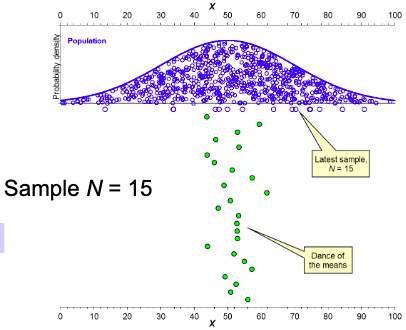
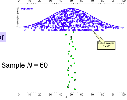
When we have a large N in the dance of the Mean

• Larger sample N usually comes closer
to estimating μ, so the dance is
narrower.

• Smaller samples vary more
dramatically.

In the Dance of the Mean

• Because of sampling variability, we
can expect to see a range of means—
however, they generally stay within a
reasonable range around μ.

You’ll that the mean heap is

normally distributed; In other words, it
has a mean and a SD like any other
normal distribution.

The mean heap is referred to as the 

sampling distribution of sample
means

What is the SD of the sampling distribution of the sample mean

The standard error of the mean (SEM)

The standard error of the mean (SEM) tells us

How precise our estimate of µ is

The sampling distribution of the sample mean estimates

the population mean µ

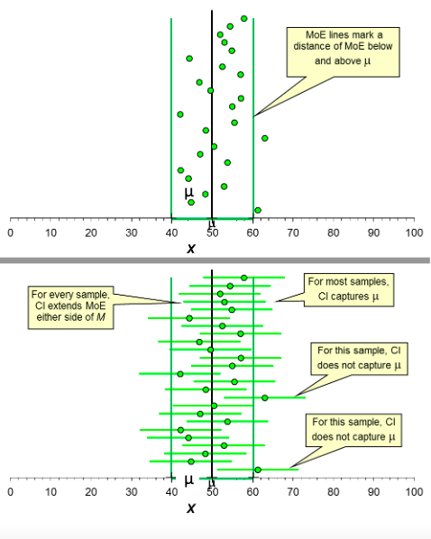
What is the Margin of Error (MoE) 

It is the combination of

1: the z- score for 95% of a normal distribution (1.96)

2: The formula for the (SEM) σ/srt of N

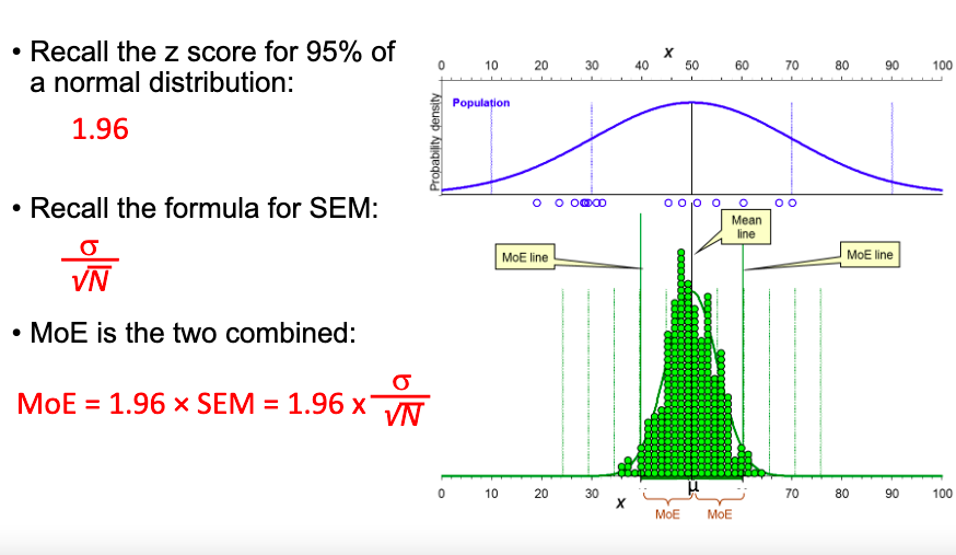
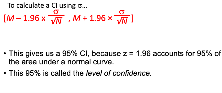
In CI, if σ is known, we can calculate it.

-Always remember, CI account the (MoE) for above & below the mean

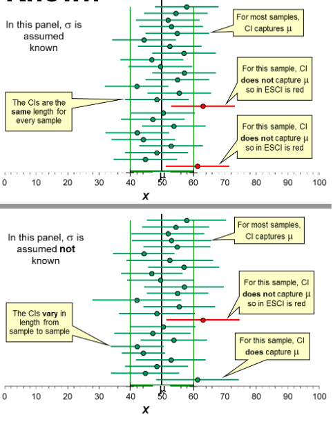
What is the dance of the CI

-the dance of the CIs tells us about the
value of μ.

• Although random sampling means
that most M values don’t equal μ,
most CIs contain μ.

Our best information about σ is in

s, the SD of our sample.

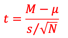
If we don’t known σ and we need to calculate the Z score, our solution is

T - scores

The t-distribution

-is very similar to the normal distribution, but with higher tails.

• This is because, not only does our estimate of μ vary from sample to sample,
but now our estimate of s does too!!

Unlike z - score that have a 1.96, t - scores have a 

2.145

Calculating the t - distribution requires a new piece of information called the

Degrees of Freedom

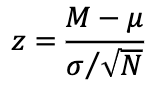
Recall that we can express estimation error of the population mean (M – μ), as a z-score:

Calculating a t-score is very similar. We simply substitute s (our sample SD) in place of s:

What is the degrees of freedom

Df = N - 1

Calculating a t-score is very similar. We simply substitute s (our sample SD) in place of s:

When σ is unknown, we replace 1.96 with tC/100 (df), and use s instead of s

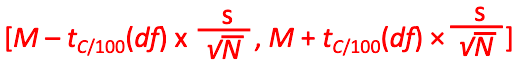
In CI when σ is not known,

However, when s is
unknown, CIs are more
dependent on s values, which
vary from sample to sample.

What are the four main approaches to interpreting the CI

1. Our CI is one from the dance
2. The cat’s eye picture helps interpret our CI
3. MoE gives the precision
4. Our CI gives useful information about replication

While we can’t know for sure if our CI gives us valuable information about μ, we always know:

• Our CI is randomly chosen from the dance

• It might include μ , and represent the dance

• It may be red, and not represent the dance

Cat’s Eye Picture

• The cat’s eye tells us about
plausibility.

• A CI has C% likelihood of
capturing μ, graphically
illustrated in a cat’s eye.

• Finding a value for μ
toward the center of CI is
more likely than finding a
value out toward the tails
or beyond.

• Be careful: even CIs with
cat’s eye pictures can still
be red—the picture only
tells us likely values of μ,
not definite.

MoE gives

Precision

MoE indicates how close our

point estimate is likely to be to μ

Higher MoE means

Lower precision

Lower MoE means 

Higher precision 

A CI can also be thought of as a

prediction interval for replication means

A replication mean is the mean obtained in a

Close Replication

Though less precise than for μ, our CI
can help us predict replication

M

The dance

Our CI is a random one from an infinite sequence, the dance of the CIs. In the
long run, 95% capture mu and 5% miss, so our CI might be red

Cat’s eye picture

Interpret our interval, provided N is not very small and our CI hasn’t been
selected. The cat’s eye picture shows how plausibility, or likelihood, varies
across and beyond the CI—greatest around M and decreasing smoothly further
from M. There is no sharp change at the limits. We’re 95% confident our CI
includes m. Interpret points in the interval, including M and the lower and upper
CI limits.

MoE

MoE of the 95% CI gives the precision of estimation. It’s the likely maximum
error of estimation, although larger errors are possible

Prediction

A 95% CI provides useful information about replication. On average there’s a
.83 chance (about a 5 in 6 chance) that a 95% CI will capture the next mean

The dominant approach to testing such hypotheses is called

null hypothesis significance testing (NHST)

What is a null hypothesis?

• The skeptical hypothesis - that there is no effect

• ”the mean IQ of U of Guelph students is equal to 100”

• What is an alternative hypothesis?

• Mutually exclusive with null hypothesis – predicts a difference!

• “the mean IQ of U of Guelph students is not equal to 100”

NHST steps:

• 1) Formulate a null hypothesis
• ”the mean IQ of U of Guelph students is equal to 100”

• 2) Collect a sample of data from population of interest
• Get a sample of U of G students and measure their IQ

• 3) Evaluate likelihood of obtaining your data if the null
hypothesis were in fact true
• Given the mean and SD in your sample, how likely is it that your
sample came from a population with a mean of 100?

p – values:

Tells us the likelihood of obtaining our result, or a
result more extreme IF the null hypothesis were true

we reject the null
hypothesis

If tobt > tcrit

we fail to reject the null
hypothesis

If tobt ≤ tcrit

The cats eye shows us that

The curve tells us that in most cases, M is close to the population mean

The cats eye picture is the

Widest or fattest at M, which tells us that most means fall close to the population mean and progressively fewer means fall at positions further away from the population mean

The cats eyes also tells us

Most likely, Mu is close to M, and likelihood drops progressively for values of Mu farther away from M, out to the limits of the CI and beyond

Where the cats eyes is the widest

It is the widest around M, which tells us that our best bet for where Mu lies is close to M

The Null hypothesis

States, for testing, a single value of the population parameter

The smaller the p value

The more unlikely are the results like ours, If the null hypothesis is true

The NHST compares

P with the significance level, often .05. If P is less than that level, we reject the null hypothesis and declare the effect to be statistically significant

Strict NHST requires 

The significance level to be stated in advanced. However, researchers usually don’t do that but use one of the a few conventional significance levels

the significance level

Is the criterion for deciding whether or not to reject the null hypothesis. If the p value is less than the significance level, reject, if not then don’t reject

If P> .05

the null hypothesis was not rejected, p > .05

If p< .05 (but p>.01)

the null hypothesis was rejected, p<.05 or rejected at the .05 level

If p <.01 (but p>.001)

The null hypothesis was rejected, p <.01 or rejected at the .01 level

If p <.001

The null hypothesis was rejected, p,.001 or rejected at the .001 level

Why .05 and not 0.05

That’s apa style for a quantity

A lower significance level (.01 rather than .05)

Requires a smaller p value, which provides stronger evidence against the null hypothesis

If using NHST

Report the p value itself (e.g., p = .14), not only a relative value (e.g., p> .05)

For the .05 significance level,

Reject the null hypothesis if it’s value lies outside the 95% CI>

If inside, don’t reject

The further our sample result, the CI, falls from the null hypothesis value

The smaller the p value and the stronger the evidence against the null hypothesis

The plausibility picture illustrates

How strength of evidence varies inversely with plausibility of values, across and beyond the CI

Prefer Hypothesis Evaluation for a fuller 

More useful interpretation than only a yes and no reject or don’t reject decision 

Hypothesis Evaluation

Focuses on interpretation in terms of strength of evidence or degrees of plausibility, rather than merely rejecting or not rejecting a hypothesis

The Null hypothesis is

H₀ and the null hypothesis value is of the population mean is µ₀

The p - value

is the probability, calculated using a stated statistical model, of obtaining the observed result or more extreme, if the null hyposthesis is true

What do we use to calculate the p value when we are willing to assume σ is known

Z

Z score when H₀ is true

Z = (M - µ₀) / σ/ str N

A test statistic

Is the statistic with a known distribution, when H₀ is true, that allows calculations of a p value

If a 95% CI falls so that μ₀ is about one -third of MoE beyond a limit

p = .01, approximately

As our mean moves farther away from the population mean

Our P value begins to lower as well

P > .05

So the CI must extend past μ₀.  the larger the P, the further the CI extends past μ₀

P < .05

So the CI extends only part way towards μ_{0, the smaller the p, the shorter the CI in relation to} μ₀

If p >.05, the 95% Ci

extends past μ₀ and the larger the p, the further it extends.

If p< .05

The CI doesn’t extends as far as μ₀ , and the smaller the p, the shorter the CI

Eyeballing the CI 

May be the best way to interpret a p value. 

If p is around .05, the CI extends from M to close to μ₀

Dichotomous thinking

Focuses on two mutually exlusive alternative.

the dichotomous reject or don’t reject decisions of NHST tend to elicit dichotomous thinking

Estimation Thinking

Focuses on how much by focusing on point and interval estimates

The inverse probability fallacy

Is the incorrect belief that the p value is the probability that H₀ is true

The p value 

Is not the probability the results are due to chance

That’s another version of the inverse probility fallacy

The dance of the p values

Is veru wide. a p value gives only very vague information about the dance

By convention, stars are used to indicate strength of evidence against H₀

1: P <.001, ***

2: P<.01 **

3: P<.05 *

The p value

Gives no indication of uncertainity

The alternative hypothesis H₁ states 

There is an effect

the alternative hypothesis

Is a statement about the population effect that’s distinct from the null hypothesis

A type 1 error

Is the rejection of H₀ when its true

False Positive:

type 2 error

Is failing to reject H₀ when it’s false

False negative or miss

type 1 error rate (a)

Is the probability of rejecting H₀ when it is true.

Not the probability that H₀ is true 

type 2 error rate (β )

Is the probability of failing to reject H₀ when it is false

False negative

A one tailed p

values indicates values more extreme that the obtained results in one direction

the direction having been stated in advance

When using means

One tailed p is half of two tailed p

A two tailed p

value includes values more extreme in both positive and negative directions

A one sided or directional alternative hypothesis

Includes only values that differ in one direction from the null hypothesis value

One tailed p includes

Values more extreme than the observed result only in the direction specified by the one sided, or directional alternative hypothesis H₁

Target Moe

Is the precision we want our study to achieve

Larger N gives 

Smaller Moe, and thus higher precision

Precision for planning

Bases choice of N on the MoE the study is likely to give.

Consider N for various values of your target MoE

The MoE distribution

illustrates how MoE varies from study to study

Increases n from 50 to 65 and, on 99% of occasions

the MoE will be less than or equal to a target MoE of 0.4

Assurance 

Is the probability, expressed as a % that a study obtains MoE no More than target MoE

For precision for planning

use Cohen’s d

Assumed to be in units of a population SD

A replication should usually have N

at least as large as the N of the original study, and probably larger