4: Dimensional Analysis by Statistical Analysis

Probability Function

Random variable X, f(x_i) = Pr(X = x_i)

Dense Sampling Set

A sampling space that’s uncountable and continuous.

Probability Density Function

For every closed interval x_i = [a, b], where for all x, f(x) >= 0 and the integral of f(x) between negative infinity and infinity is 1.

• S is a dense sampling space

• Powerset(S) = {c_i} and the powerset of all subsets of S

• X: S → T is a dense random variable defined over S where T = {x_i} and X(c_i) = x_i

Probability Density Function Properties

• For all x, Pr(X = x) = 0

• P(X >= a) = integral between infinity and a of f(x)

• P(X <= a) = integral between a and negative infinity of f(x)

Cumulative Probability Distribution Function

F(x) = P(X <= x)

• X is a random variable defined over a sampling space

Cumulative Probability Distribution Properties

• Always increasing but not always monotonic - x₁ < x₂ → F(x₁) <= F(x₂)

• lim(x → -inf.) F(x) = 0 and lim(x → inf.) F(x) = 1

• Pr(X > x) = 1 - F(x)

• x₁ < x₂ → Pr(x₁ < X <= x₂) = F(x₂) - F(x₁)

  • Note - F(x) is only continuous on the right-hand side, but not always on the left

Joint Distribution

A collection of probabilities over a series of random variables’ sampling spaces: Pr(X₁ = c_{x1, j}, …, X_n = c_{xn, k})

• X are the random variables

• n is the number of random variables

• Powerset(X_i) = {c_xi}

• j and k indicate elements in x

Denoted as f(x, y)

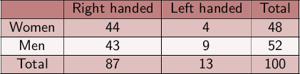
Bivariate Distribution

Joint distribution where n = 2 (i.e. there are two random variables)

Contingency Tables

Frequency matrices that express joint frequences for 2 or more categorial variables.

Mutual exclusion (Disjoint)

• Where two sets never contain common outcomes (A ∩ B = {}).

• For more than two sets, for each pair of sets denoted by i, j where i ≠ j, A_i ∩ A_j = {}

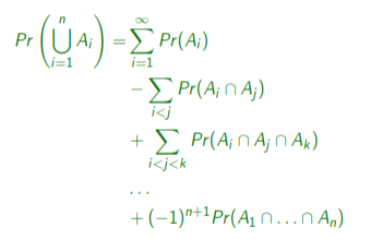
Probability of a union of events

Probability of a union of disjoint events

Just a sum of all individual probabilities.

Probability of a union of two sets

P(A ∩ B) = P(A) + P(B) - P(A U B)

Independence of two sets

P(A ∩ B) = P(A) * P(B)

• The occurrence of one event does not give us information about another event.

Statistically Independent Random Variables

The joint probability distribution function is factorisable in the form P(X, Y) = P(X) * P(Y)

Information contained in the occurrence of an event

I(e_i) = -log_b(P(e_i)) = log_b(1/P(e_i))

Units of information

Depends on the base used:

• Bits if 2

• Hartleys if 10

• Nats if e

Entropy

The average amount of information you get from the source - a measure of uncertainty.

• Affected by statistical independence

• The more common the event is, the less information it carries

Information (r.e. Entropy)

Resolves uncertainty, tells us more about a random variable.

Entropy Formula

H(X) = For all i, P(x_i) * I(x_i) = -(for all i, P(x_i) * log_bP(x_i))

Joint Entropy Formula

H(X, Y) = -(for all x_i in X (for all y_j in Y (P(x_i, y_j) * log_bP(x_i, y_j))))

Independent Component Analysis

Used to decompose a signal into statistically independent sources (bases).

• In the formula Y = XB, ICA solves for both X and B at the same time.

• Mathematically solving X ~= X^ = WY, W ~= B^-1

• Only produces approximations

Independent Component Analysis Formula (Long)

• Observe J linear mixtures y₁, … y_j comprised of I = J sources x₁, …, x_i

• For all j in J, B_{(1, j)}x₁ + B_{(2, j)}x₂ + … + B_{(i, j)}x_i

Independent Component Analysis Formula

Y = XB = for all i in I (sources), B_{(i, j)}x_i

Independent Component Analysis Limitations

• Always assumes the components are mutually independent, mean-centred and have non-Gaussian distributions

• Cannot identify the number of source signals or the proper scaling of them

• Ignores sampling order (time dependency) and works over variables rather than signals

Solving for an estimation - assumption (ICA)

That the sources are mutually exclusive.

Solving for an estimation (ICA)

Maximising the joint entropy of X^, i.e. g(X^) = g(WY)

• g(X^) is the cumulative density function of X^

• Independence of sources is obtained by adjusting the mixing of W ~= B^-1

• This also maximises the mutual entropy, H(g(X^))

• Then use gradient descent to take a small step in the direction of the gradient of H(g(X^))

• W_new = W_old + h * gradient(H(g(X^)))

  • h is the learning rate