Producer Theory

Producer Theory

Production: Inputs → outputs

• Goal: Profit maximization/cost minimization

Assumptions: 

• The firm produces a single good

• The firm has already chosen which product to produce

Profit (π) Formula

= Total Revenue (TR) – Total Cost (TC)

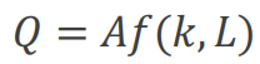
Production Functions

(comparing to utility functions)

Inputs: 

• Labour 

• Capital 

Output: q 

Production function: q=f(L, K) 

More assumptions: 

• The more inputs the firm uses the more output it makes

Variable Input (Labour)

can be changed in the short run

Fixed Input (Capital)

can’t be changed in the short run

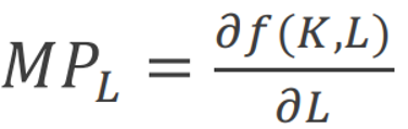
Marginal Product of Labour (MP_L)

the additional output the firm can produce by using an additional unit of labour (keeping the capital fixed)

Diminishing Marginal Product of Labour

As a firm hires additional units of labour, the marginal product of labour falls

• E.g. Even hundreds of workers will make little progress digging a hole if they have no shovel to dig with

• In the short run capital (shovel) is fixed

Long run Production Decisions

Trade off between L and K (comparing to trade off between pizza and coke)

Isoquants (comparing to indifference curves)

Cobb-Douglas

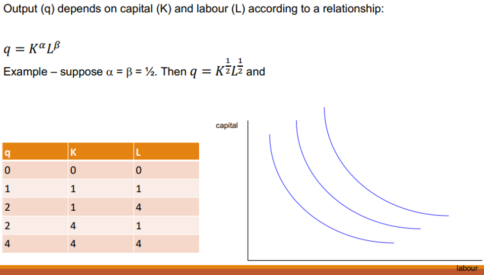
Isoquants

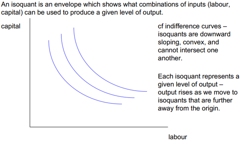
What does a Higher Isoquant mean?

higher output level

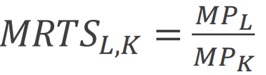
Marginal Rate of Technical Substitution (MRTS_L,K)

the rate at which the firm can trade labour (L) for capital (K), holding the output constant

it’s the (negative of) slope of the isoquant

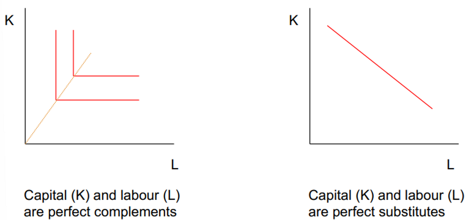
Special Cases of Isoquants

Returns to Scale

a change in the amount of output in response to a proportional increase of the inputs

Constant Returns to Scale

happens if changing the amount of capital and labour by some multiple changes the quantity of output by exactly the same multiple

doubling labour and capital doubles output

Increasing Returns to Scale

happens if changing the amount of capital and labour by some multiple changes the quantity of output more than proportionally

doubling labour and capital more than doubles output

Decreasing Returns to Scale

happens if changing the amount of capital and labour by some multiple changes the quantity of output less than proportionally

output does not fully double when inputs are doubled

Technology Change (Total factor productivity growth)

an improvement in technology that changes the firms production function such that more output is obtained from the same amount of inputs

Cost Formulae

• Total cost = fixed cost + variable cost

• Fixed cost – fixed input — capital – r (rental rate)

• Variable cost – variable input — labour – w (wage rate) 

What determines the shape of Total Costs in the Short-Run?

the law of diminishing marginal product

Average Costs

total cost / output

in the short run it will decrease at first as the fixed cost needs to be spread - as you produce more it will increase

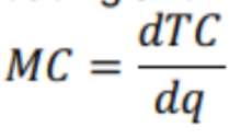
Marginal Cost

the cost of producing another unit of output

Long Run Cost Minimisation

firms choose K and L to maximise production efficiency

cost minimization: economically efficient input combination for a given q

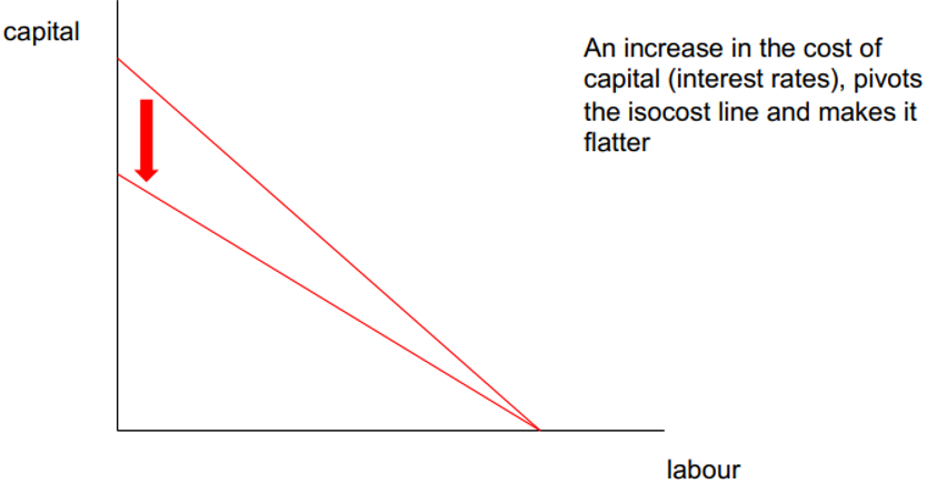
Isocost lines (comparing to budget constraint)

Cost = V(K) + W(L)

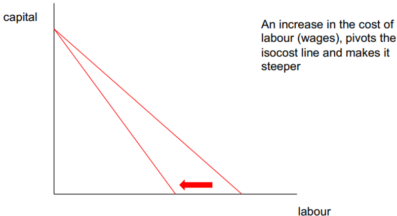
Isocost Lines

shows what combinations of the two inputs can be employed for a given cost

Isoquants and Isocost Lines

shows what combinations of the two inputs can be employed for a given cost

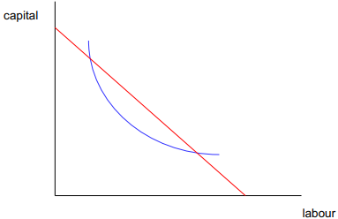
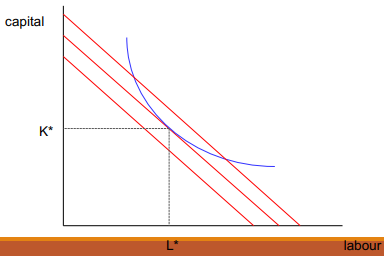
Isoquants and Isocost Lines: Cost Minimisation

tells us how cheaply it is possible to produce a given level of output – and what is the best combination of inputs to use

The key point is at tangency between a given isoquant and the lowest attainable isocost line

MRTS = w/r

Conditions (comparing to optimal consumption)

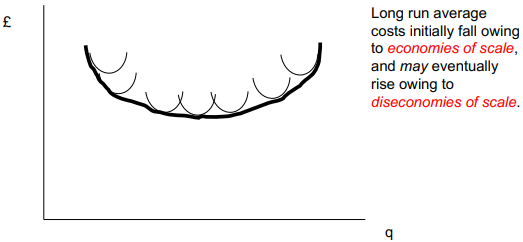
Cost Curves in the Long Run

In the long run, firms can vary the amount of capital they employ. They can therefore shift onto different short run cost curves. Owing to economies of scale, and subsequent diseconomies of scale, the long run average cost curve is an envelope around short run average cost curves:

The long run marginal cost curve passes through the minimum of the long run average cost curve

Economies of Scale

if doubling output causes cost to less than double

total cost rises at a slower rate than output rises

may be due to: fixed costs; specialisation; quality of machinery

Diseconomies of Scale

if doubling output causes cost to more than double

total cost rises at a faster rate than output rises

may be due to: managerial diseconomies / bureaucracy; geographical diseconomies

Constant Economies of Scale

if doubling output causes cost to double

total cost rises at the same rate as output rise