Financial econometrics - theory

advantage of cash

• liquidity

disadvantage of cash

• subject to inflation/devaluation

advantage of having percentage of GDP when talking about volume of trade

• global GDP is growing, it is better to standardized somehow

• using the dollar is subject to inflation so this will result in skewed results

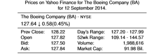
What do these numbers mean?

• 127.64 is the last price the share was slod at

• 0.58 is the different in the current trade and the previous close (it is lower)

• the first trading price of the day was 127.82

• we mainly use the closing price for empirical work

what does a smaller bid-ask spread result in?

• high levels of liquidity

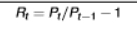
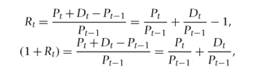
formula for 1-period simple return

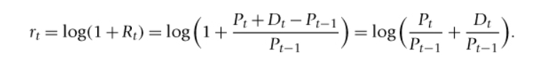
formula for 1-period log return

formula for k-period simple return

• the operator on the right hand side is the product operator

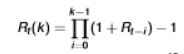
formula for k-period log return

• we simply aggregate the log returns which we can’t do with simple returns as we have to compound it ourselves

• simply the sum of the single period log returns over the period

formula for annualised simple return

• useful when we have two returns measured in different frequencies

• assume monthly returns will persist for 12 months

formula for annualised log return

• useful when we have two returns measured in different frequencies

• assume monthly returns will persist for 12 months

formula for portfolio simple return

• simple is preferred to log as it is additive

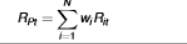
formula for annualized log return

is a dollar return scale-free?

• no

examples of price-weighted indices

• dow jones industrial average index (dow jones/DJIA) (US)

• Nikkei 225 index (Nikkei/NKX) (Tokyo)

examples of value-weighted indices

• Deutscher Aktien Index (DAX) (Germany)

• Financial Times Stock Exchange 100 Index (FTSE) (UK)

• Hang Seng Index (Hang Seng/HSX) (Hong Kong)

• Standard and Poors Composite 500 (S&P 500)

stylised facts about financial data

• heavy tails (measured by kurtosis (4th movement))

• asymmetry (measured by skewness (3rd movement))

• we use t-distribution for financial data

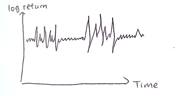
• volatility clustering

• departure from normality

• long-range dependence (2nd order dependence)

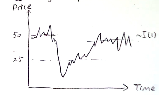
• log price of an asset is typically an integrated process

• some series of the log prices of assets keep co-movement in long run but some trending variables can have spurious (not genuine) relationships

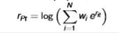
details about heavy tails in financial data

• the density of asset returns has heavier tails than normal

• there is excessively high proportion of extreme values

• distribution is still centred/symmetric but the probability of extreme values is higher than normal

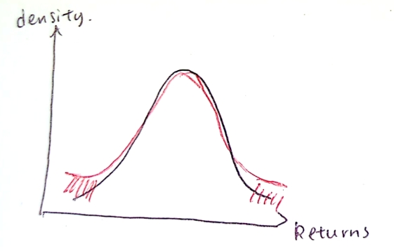
details about asymmetry in financial data

• the density of asset returns is slightly negatively skewed

• there is higher proportion of negative returns than positive returns

• more likely to get a negative return than a positive return

• earnings could be positively skewed (skewed to the right)

details about volatility clustering in financial data

• large changes in log price comes in clusters

• this issue has been extensively studied in ARCH (autoregressive conditional heteroskedasticity) literature

• periods of high volatility tend to follow high volatility periods

• periods of low volatility tend to follow each other

• we observe period of low volatility, periods of high volatility, periods of low volatility, etc.

details about departure from normality in financial data

• high frequency asset returns show obvious departure from normality

• the distribution of asset returns at other frequencies also tends to be non-normal

details about long-range dependence in financial data

• one observes strong serial correlation in variance (not mean) of returns

• r²t or IrtI is strongly autocorrelated

• this feature may help explain volatility clustering

details about log price of an asset being an integrated process in financial data

• many such series appear to have upward trends

• such series commonly have unit roots, which affect inference

• mean and variance are not constant over time

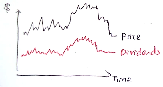
graphical representation of co-movement of prices and dividends

• not moving at the same level but their movements are very similar

• if they are both I(1) processes, we could model them together to make a stationary process

• could model how they would move in the long-run

if prices are exponential, what do we expect log prices to be?

• linear, growing at a constant rate

• if log prices are linear, we expect log returns to be constant

• Pt - Pt-1 = some constant

do we expect returns to follow a leptokurtic or platykurtic distribution?

• leptokurtic

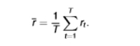
formula for mean

• 1st moment - where is the distribution centred?

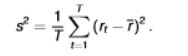
formula for variance

• 2nd moment - how spread out is the distribution?

formula for skewness

• 3rd moment - is the distribution symmetric?

• SK < 0 = negatively skewed, SK >0 = positively skewed

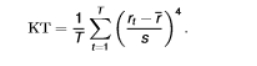
formula for kurtosis

• 4th moment - the tail behaviour of the distribution

• we compare this to the value KT = 3 as this is the kurtosis value of a normal distribution

formula for excess kurtosis

• distribution with positive excess kurtosis is leptokurtic

• distribution with negative excess kurtosis is platykurtic

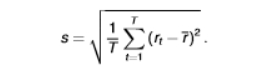
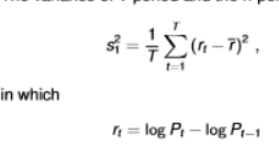
formula for volatility

• also the formula for sample standard deviation which is the square root of the sample variance

• variance will be non-zero and positive (as it is squared)

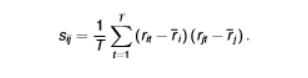
formula for sample covariance

• we use this when we have two time-series

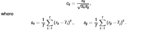
formula for sample correlation

• value will range between -1 and 1

• if the correlation = 0, the assets are linearly independent

when there are large outliers, is the median or the mean preferred?

• the median

• if we used the mean, the outlier would skew the mean calculation

which percentiles of distribution are important in finance?

• the 1st and 5th percentiles to measure the value at risk

why do we need to calculate VaR?

• the financial system can become less stable when huge losses are suffered by financial institutions in the system

• we measure the potential loss faced by banks to reflect financial sector stability

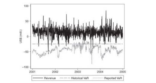
example of value-at-risk

• the 1% value at risk for the next h periods conditional on information at time T is the 1st percentile of expected trading revenue (which can be a gain or a loss) at the end of the next h periods

• if the daily 1% value at risk is $30 million, there is a 1% chance the bank will lose $30 million or more after 1 day

• although $30 million is a loss, by convention, the value at risk is quoted as a positive number

historical simulation for computing VaR

• the historical method simply computes the percentiles of the empirical distribution from historical data

the variance method for computing VaR

• the method assumes that returns are normally distributed

• we use 2.33 as it is a one-sided test (calculating the loss so just looking at the left tail of the distribution)

• where ɥ and σ are the sample mean and standard of the returns (respectively)

monte carlo simulation for computing value-at-risk

• involves simulating a model for returns several times and constructing simulated percentiles

• using a model to make forecasts of future values of the asset or portfolio and then assessing the uncertainty in the forecast

what does 1% VaR mean?

• you would hope 1% falls below your prediction

• if below 1% falls below your prediction, you are very conservative

autocorrelation formula

• it is similar to the correlation formula

• only applied to one variable and its own lag, instead of two variables

• the numerator represents the autocovariance of returns k periods apart

• the denominator represents the variance of returns

if EMH is true, what does it imply?

• the current price of an asset reflects all relevant information available on the market

• the current price provides no information regarding future asset movements

• future returns are completely unpredictable, given information on past returns

• traders cannot systematically use newly arriving information to make a profit

• conditional on all previous information, returns are completely random

what does zero autocorrelation imply?

• returns exhibit no predictability

• EMH exists

• future movements in returns are unpredictable in terms of their own past history

• foreign exchange rate is considered to be efficient as the autocorrelation ~ 0

if returns exhibit positive/negative autocorrelation, what does this imply?

• this pattern can be exploited to predict future behaviour

• EMH is violated

variance ratio of 1-period

• alternative way to examine the EMH

• we are comparing the variance ratio on returns over different time horizons

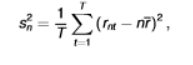
variance of n-period returns

• nr(~) = sample mean of the n-period returns rnt

• alternative way to examine the EMH

• we are comparing the variance ratio on returns over different time horizons

how do we construct the variance ratio?

• we first impose that the variances rt, rt-1, rt-2,…, are the same and do not depend on t

• we are imposing the assumption of homoskedasticity for this to work

if there is no autocorrelation, what does the variance of n-periods equal to?

• the variance of n-period returns should equal n times the variance of the 1-period returns

• the ratio is known as the variance ratio

significant values for the variance ratio

• = 1 means no autocorrelation

• >1 = positive autocorrelation

• <1 = negative correlation

• if we have VRn = 0.99, we would have to conduct a hypothesis test as we can’t assume there is no autocorrelation just because the value is close to 1

limitations of autocorrelation

• not a universal measure of predictability

• can capture, at most, linear predictability of mean returns

• possible for us to extend the concept of autocorrelation to measure predictability of higher moments such as variance, skewness, or kurtosis

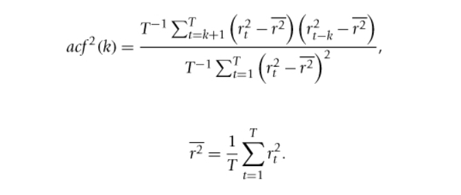
autocorrelation in squared returns formula

characteristics of autocorrelation in squared returns

• we can have negligible acf(k) and sizeable acf²(k)

• this is case, the mean is not predictable but the variance is

• this does not violate the EMH as it is only concerned with the expected value of returns, and not their variance (or higher moments)

• in fact, many functions of returns can display predictability, in terms of autocorrelations

why do we need to use financial econometrics?

• hope to help regulators and policy markers to be better equipped to assist in monitoring markets toward the goal of financial stability

• also to guide the smooth functioning of financial markets in the face of crisis

• distinguishing feature is that there is an abundance of financial data

how can foreign exchange be seen as a cash investment?

• the exchange rate is simply the price of one currency in terms of another

the use of summary estimates of prices

• we are increasing the number of observations

• does not always increase the efficiency or improve understanding

the effect of a dividend payment

• to lower the share price by the amount of the dividend

• the closing price of the previous day is greater than the opening price of the following day

• process of adjustment does not mean that historical prices reflect the actual prices at which trades took place

adjustment for a 2-for-1 stock split

• a company replaces each existing share by two shares

• the price of the share is immediately halved

• makes the shares look more affordable, even though the market capitalization of the company has not changed

• to make the prices before and after the split comparable, all historical prices need to be divided by 2 and the historical volume series needs to be multiplied by 2

disadvantages of dollar returns

• not scale-free

• does not measure the return relative to the initial investment

• depends on the unit in which prices and dividends are quoted

simple gross return formula

• rearranged the simple return formula

• useful to represent the value at time t of investing $1 at time t-1

are simple returns additive when computing multi-period returns?

• no

• due to the multiplicative effect of period-by-period returns

• whereas log returns are continuously compounded returns

what is the significance of e=2.17828 for log returns?

• represents the value of an account at the end of year that started with $1 and paid 100% interest per year but the interest compounded continuously over time

how many trading days are there?

• approximately 252 (due to public holidays/leap year)

are continuously compounded returns similar to simple returns?

• only if the return is small

• generally the case for monthly and daily returns

simple and gross returns with dividend payments formulae

• Dt/Pt-1 = dividend yield

log returns with dividend payments formula

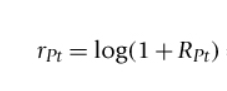
log return on a portfolio

• = Rpt when Rpt is small

• Rpt = portfolio rate of return which is equal to the weighted average of the returns to the assets

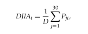
formula for Dow Jones index

• D = Dow Jones divisor

advantages and disadvantages of price weighting

• + simplicity

• - stocks with the highest price have a greater relative impact on the index than they perhaps should

• - the price-weighted index overemphasised market movements during the period of the dot com bubble, as well as the speed of the recovery form the 2008 global financial crisis

disadvantage of value weighting

• securities whose prices have risen the most (or fallen the most) have a greater (or lower) weight in the index

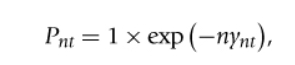
price of zero-coupon bond

• the right hand side is the discounted present value of the principal

• -ny_nt= discount rate

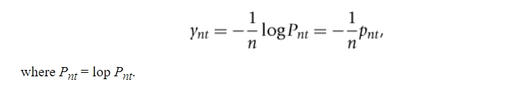
yield on a zero-coupon bond

• the yield is inversely proportional to the natural logarithm of the price of the bond

• -1/n = constant

features of yield curves

• at any point in time when the yield curve is observed, all the maturities may not be represented

• this is particularly true at longer maturities where the number of observations yields is much sparser than at the short end of the maturity spectrum

• the yields at longer maturities tend to be less volatile than the yields at the shorter end of the maturity spectrum

• the shape of the yield curve is determined by the demand and supply of the bonds of various maturities, market expectations, and risk assessments

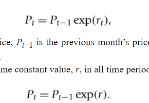
formula for exponential pattern in stock prices

• Pt = current equity price

• Pt-1 = previous month price

• rt = rate of the increase between month t-1 and month t

• the second equation shows if we restrict rt to take the same constant value

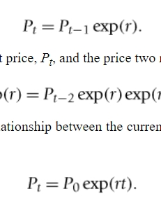
general formula for the relationship between the current price and the price t months earlier

• rt = how many months between the two prices

• the second equation is derived when we take the natural logarithms

what is the effect of measuring returns over very short periods of time?

• any tendency of prices to drift upward is virtually imperceptible as the effect is so small and is swamped by the apparent volatility of returns

• returns generally focus on short-run effects whereas price movements can trend noticeably upward/downward over extended periods of time

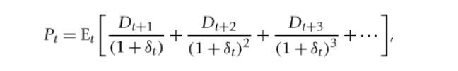
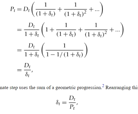
the present value model formula

• where dt = discount rate (on denominator)

• the price of an equity is equal to the discounted future stream of dividend payments

• results in deriving the yield curve (last line)

• the relationship between equity prices and dividends is upward exponentially trending, with stronger intermittent downturns for equity prices

• can change the property by combining two or more series

natural logarithms equation of the present value model

• reveals the linear relationship between logPt and logDt

3 important properties of yields of zero-coupon bonds

• yields are increasing over time, so they exhibit some form of trending behaviour

• the variance of the yields tends to grow as the levels of the yields increase (levels effect)

• yields of different maturities follow one another closely

important distinguishing feature of transactions data

• the time interval between trades is not regularly/equally spaced

• if high-frequency data are used, there will be period where no trades occur and the price won’t change

an example when the sample mean is an inappropriate summary measure

• when the data are trending

how does positive/negative skewness change the shape of the distribution?

• positive skewness = heavier right tail

• negative skewness = heavier left tail

properties of correlation

• has the same sign as the covariance

• lies in the range -1</= cjj </= 1

• not unit dependent as the measurement units are scaled out

VaR example

• if the daily 1% h-period VaR is $30mil, there is a 1% chance that the bank will lose $30mil or more

difference of the VaR computed from the variance method and the historical method

• the value computed from the variance method is slightly lower than that computed by historical returns as the assumption of normality ignores the slightly fatter tails exhibited by the empirical distribution of daily trading revenues

ways to use sample statistics to test the efficient market hypothesis

• test asset returns for predictability

• compare the variance of asset returns over different time horizons

autocorrelation of returns reveal information about the temporal dependence properties of the levels of returns

• reveals information about the autocorrelation properties of the squared levels of returns

if the squared level of returns are predictable, does this violate EMH?

• as long as the level of returns are not predictable, this does not violate EMH

• EMH is only concerned with the expected value of the level of returns

various power transformations of returns computed by autocorrelation

• first one = skewness

• second one = kurtosis

• third one = the absolute magnitude of returns (alternative measure of the presence of autocorrelation of variance)

• last one = general power transformation

• if a = 0.5, this is the autocorrelation of the standard deviation

what does the presence of stronger autocorrelation in squared returns than returns themselves suggest?

• it suggests that other transformations of returns may reveal even stronger autocorrelation patterns

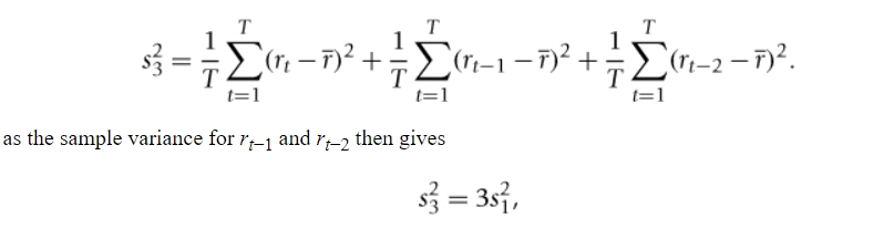
proof that a variance ratio of 1 means no autocorrelation

• we are using an n=3 period return

• sum of the three 1-period returns in the first equation

• r(-) = sample mean for the 1-period return

• we square both sides and average over a sample size T which gives what we see in the picture

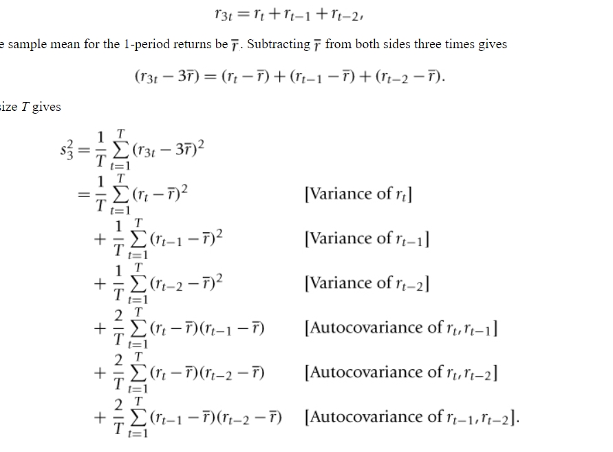
in the case of zero sample autocovariances, what does the variance ratio relationship simplify to?

• the second equation shows if we assume the sample variance for rt is the same as the sample variance for rt-1 and rt-2

• there is no sample autocorrelation in the n=3 period return

• this falls under the covariance stationarity assumption

does regression always capture causal relationships?

• no

• for example, we could find an increase in ice cream sales and an increase in crime rates (spurious relationship)

• predictive regression, ie yt = monthly indicators

• being in december doesn’t explain migration but having the december indicator can help us to predict net migration in that month

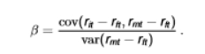
CAPM formula (in terms of beta risk)

• describes the risk characteristics of an asset in terms of B-risk

• r_it - r_ft = the return on asset i relative to the risk-free rate r_ft (excess return)

• r_mt - r_ft = market return relative to the risk-free rate

• we can use the treasury bill rate as r_ft and S&P 500 returns as r_mt

• the numerator is the covariance between the excess returns on the asset and the market and the denominator is the variance of the market

• the expression is the same as the slope estimate for simple linear regression where cov(y,x)/var(x)

what is the support of beta in the CAPM?

• it is on the real line

• covariance is unbounded

• variance is non-negative and unbounded

• the relative magnitudes of the covariance and variance are unclear to us so beta could take any value from -∞ to ∞

how are individual stocks or portfolio stocks classified?

• in terms of their degree of B-risk

• moving in the same direction as market = aggressive, benchmark, conservative

• moving in the opposite direction as the market = imperfect hedge, perfect hedge

• when beta is positive, it follows the same direction as the market (benchmark)

• when beta is negative, it moves in the opposite direction as the market (hedge)

• B= 0 when there is no covariance so the numerator is zero (the assets are independent)

• ie if r_it = r_ft

• the denominator cannot be zero as this means it is constant

• the covariance between a variable and some constant is always zero

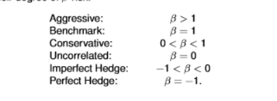
with which type of beta risk do we earn the market return?

• benchmark

• beta = 1

with which beta-risk do we earn the risk-free return?

• uncorrelated

• B = 0

• this means that it is independent of the market

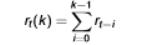
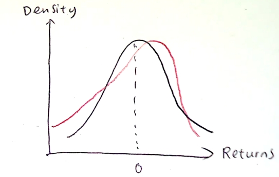
how do we estimate beta?

• we use the linear regression model

• the disturbance term ut captures additional movements in the dependent variable not predicted by CAPM

• if we did not include this, we would assume the regression is perfect; no unobservables at all

• we assume zero conditional mean, that is E[ut Irmt - rft] = 0 (we have removed the market factor already)

• we prefer a positive alpha (we want to earn that little bit extra compared to the market

• two unknowns:

• the intercept parameter a captures the average abnormal returns to the asset given the relative risks

• the slope parameters B corresponds to the asset’s beta-risk

• rit - rft = the excess return on asset (dependent variable)

• a = captures the abnormal return to the asset over and above the asset’s exposure to the excess return on the market

• if a>0, the asset earns higher (abnormal) returns in excess of the return predicted by CAPM

• if a<0, the asset earns lower (abnormal) returns in excess of the return predicted by CAPM

• b = beta risk

• rmt - rft = excess return on market (explanatory variable)

• ut = captures additional movements in the dependent variable not captured by CAPM