Applied econometrics 2 lectures 1-4 - Time series regression

Time series data

consist of observations on a given economic unit (e.g. a country, a stock market, a currency, and an industry) at several points in time with a natural ordering according to time

Frequency

The length between two successive observations

high vs low frequency

The more high frequency the data is, the more observations are taken. E.g. monthly is more high frequency to yearly

The signal

The systematically predictable component of the time series

What does the signal consist of

The signal consists of three major components: trend, seasonal and cycle. A given time series may incorporate some or all of these components

The signal - trends

the persistent tendency (if any) of the time series to increase or decrease over time.

o Trends may change over time both in magnitude and direction

The signal - Seasonality

a type of cyclicality where the time series has a tendency to increase or decrease in predictable or regular ways

o E.g. at the same quarter of year or the day of the week. This gives the time series a smoothly oscillating character.

o Often series that display seasonal patterns are seasonally adjusted before being reported for public use

The signal - cycles

When a time series oscillates around a trend

o The timing and duration of oscillations of cycles however can often tend to be irregular or aperiodic

Lagged variable

the observation in the previous period being used (t-1)

Difference variable

the difference between the current value of the variable and its value in period t-1

• With X measured in logs, the first difference would give the proportional (%) change in X between period t-1 and t

Stationarity

A variable that trends back to the same mean

if I look at different same-length “chunks” of the time series, they should look similar

Nonstationary

A variable that doesn’t tend to go back to the same mean

Stationarity in economics

In general, most macro and financial variable are nonstationary, but their first differences (or returns) tend to be stationary

Stochastic process / time series process

sequence of random variables indexed by time

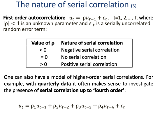
(1st) Autocorrelation / serial correlation

Correlations involving a variable and its own (1st) lag

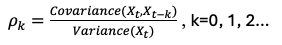
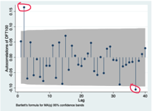
Autocorrelation function (ACF / correlogram)

gives a sequence of autocorrelations across different lag lengths / orders

• Autocorrelations measure the strength of linear association between two variables → Lies between -1 (perfectly negatively correlated) and 1 (perfectly positively correlated).

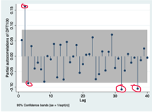
partial autocorrelation function (PACF)

the correlation conditional on all other autocorrelations in between - net correlation

PACF between X_t & X_t-3 includes order 1&2

Dynamic relationship

where a change in a given variable X today, has impact on that same variable or other variables in one or more future time periods

Static model

An explanatory variable x only has a contemporaneous impact on y

y_t = f(x_t) + u_t

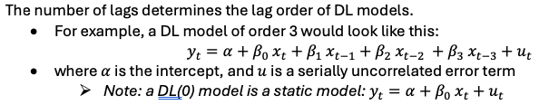
finite distributed lag (DL) model

A dependent variable y is a function of current and past values of an explanatory variable x but not its own past values

y_t = f(x_t, x_t-1, x_t-2, …) + u_t

Lags of x impact y

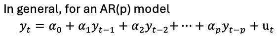
autoregressive (AR) model

A model exclusively made up of lagged dependent variables as explanatory variables

y_t = f(y_t, y_t-1, y_t-2, …) + u_t

a regression of y on its own lags

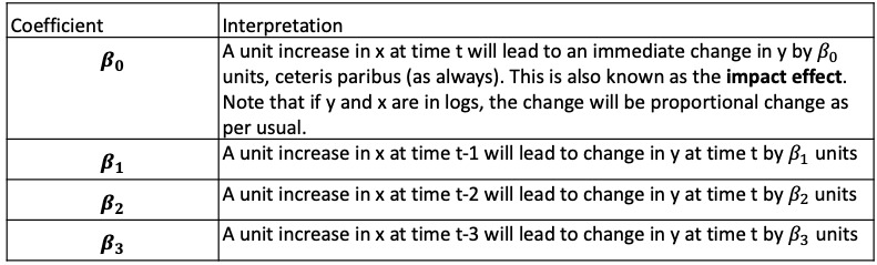
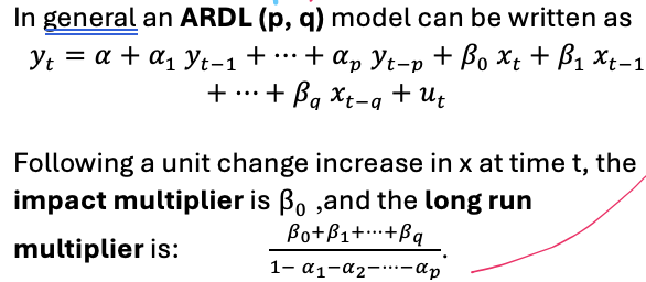
autoregressive distributed lags (ARDL) model

A combination of models DL and AR

y_t = f(y_t, y_t-1, y_t-2, … , x_t, x_t-1, x_t-2, …) + u_t

Y is impacted by its past self and current + past of other variables

If you include 1 lag of y and 2 lags of x you have the ARDL (1, 2) model

Effect of a temporary increase in x - DL model

Suppose x_t increases to x_t +1 temporarily

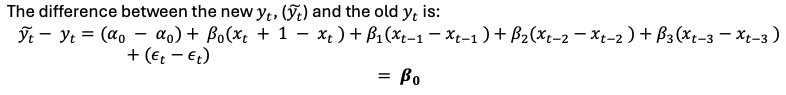
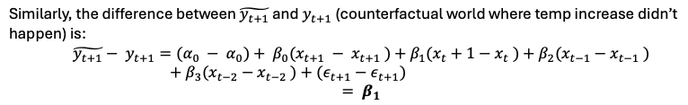
impact multiplier DL model

β₀ – what happens to yt today if xt changes by 1 unit today

Lag distribution

All β_j‘s as a function of j

Found when finding the difference between real and counterfactual for all future periods - summary of the dynamic effect on y of a temporary increase in x.

B0 impact today + B1 impact tomo + B2 impact 2 days from now…

Effect of a permanent increase in x - DL model

Suppose x_t increases to x_t +1 permanently

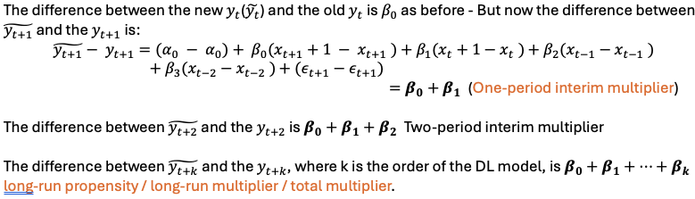
Long-run multiplier - DL model

β₀ + β₁ + … + β_k

Weak dependence

As time passes correlation falls and eventually reaches 0

All AR(1) processes are weakly dependent if |p| < 1

Asymptotic properties of OLS

TS1 - Linear in parameters and weak dependence

TS2 - Zero conditional mean (only require contemporaneous not lagged variables)

TS3 - No perfect collinearity

+ To make asymptotically normal:

TS4 - Homoscedasticity

TS5 - No serial correlation

Possible failures of OS assumptions and solutions

Failure of: TS.4 → Use heteroskedasticity-robust standard errors

Failure of: TS.2

• A possible violation could occur if both y and x are correlated with unobserved trending variables (spurious regression) → control for a time trend by adding t as a right- hand-side variable

• Seasonality → use seasonal dummies

Failure TS5 - No serial correlation

Correlation of errors and nature of correlation

If corr(u_t , u_t-k ) ≠ 0 for at some k, → serial correlation

Causes of serial correlation in errors

• Variables omitted from the time-series regression that are correlated across periods and are now lumped into the error term.

• The use of incorrect functional form (e.g., a linear form when a nonlinear one should be used).

• Systematic errors in measurement

Consequences of serial correlation - Bias

If the model contains lagged dependent variables - OLS biased on all coefficients

if no lagged variables then no bias (but inefficient)

Consequences of serial correlation - Inference

Breaks TS5 → Standard error calculation incorrect → invalid hypothesis testing procedures (t test etc.)

True with or without lagged dependent variables

Tests for serial correlation

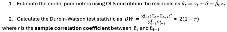
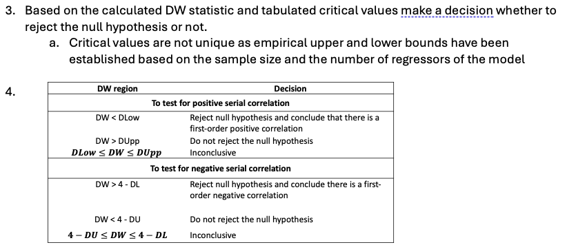
• Durbin-Watson test

  • Only Tests for first order autocorrelation

  • Not Valid if model contains Lagged dependent variables

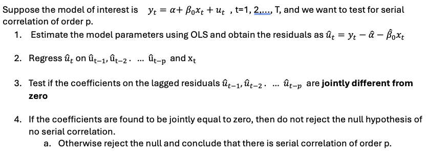
• Durbins’s Alternative test

  • Can test for higher orders

  • Can be used if model has Lagged dependent variables

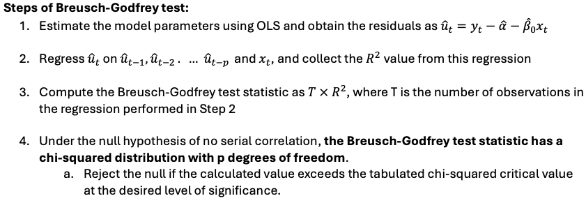
• Breusch-Godfrey test

  • Same as Durbins alternative

Durbin-Watson test (not including how to carry out)

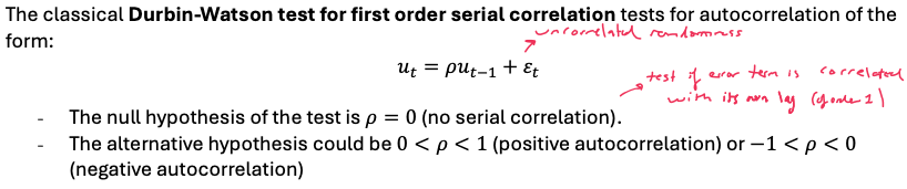
Can only be performed if regression model has an intercept + NO LDV + Autocorrelation of first order

Durbin-Watson test steps to carry out

Durbin’s Alternative test steps to carry out

Breusch-Godfrey test steps

Solutions to serial correlation

i. Fix the standard errors: Newey-West standard errors [Modern solution]

ii. Change the estimator: Feasible generalised least squares estimator [Old School]

Pros and cons of NW

• Pro

  • Robust to arbitrary form of correlation

• Cons

  • Need to specify no. lags

  • Might not be efficient

  • Does not fix bias from LDV

Pros and cons of FGLS

Pros

• Most efficient estimator (if you get it right)

Cons

• You need to correctly specify functional form of serial correlation

Newey west standard errors

If the model doesnt contain LDV, you can estimate the model parameters using OLS and then compute standard errors

• The resulting standard errors are robust to heteroscedasticity and autocorrelation

  • Known as autocorrelation consistent (HAC) standard errors.

- HAC SEs allow for unrestricted serial correlation (up to the order of the chosen lag) and heteroskedasticity

- Major advantage: serial correlation can be of any form - no need to make a precise functional form assumption.

- Con: you need to specify the number of lags in the serial correlation.

Feasible Generalised least squares estimator (FGLS) steps

1. Assume a structure in the serial correlation

2. Quasi-difference your variables

   1. Lag the original model by 1 period

   2. Multiply lagged model by p + subtract from og model

   3. rewrite model where (variable)* = og - lagged

3. The quasi-differenced model has a serially uncorrelated error (OLS works) but p is unknown

4. Estimate og model with OLS

5. regress error on lagged error for estimate of p and p^

6. use p^ to obtain initial FGLS estimate

7. Use residuals to redo step 5 + 6 until convergene in estimate of p

BG test steps

1. Estimate model

   1. Obtain residuals

2. Regress u_{t on} u_t-1 , u_t-2 … & x_j

   1. Get R²

3. BG test stat = T*R²

   1. Chi squared with p Df

   2. Null no serialcorrelation

DA test steps

1. Estimate model

   1. Obtain residuals

2. Regress u_{t on} u_t-1 , u_t-2 … & x_j

   1. Obtain coefficients

3. Test for joint significance of coefficients

   1. If = 0 then don’t reject null of NO serial correlation