Chapter 11 Income and Expenditures

Is the relationship between GDP and the multiplier NOT a 1:1 ratio?

Yes:

• Multiplier effect indicates that an initial change in spending leads to a larger overall change in GDP

T/F: what’s spent is saved

T

MPC defintion & formula

changes in spending based on some change in income; every additional dollar you make, how much do you spend of additional dollar

• the increase in consumer spending when disposable income rises by $1

change in C / change in I

If consumer spending goes up by $6 and disposable income goes up by $10,

MPC = ?

$6/10 = 0.6

MPS formula & defintion

change in S / change in Ys

• S: savings

• Ys: fraction of income saved/not spent

fraction/proportion of any change income that is saved

disposable income?

after tax

MPC + MPS =

1

total increase in real GDP formula

[1 / (1 - MPC)] * $ amount

Suppose that the marginal propensity to save in an economy is equal to 0.2. Suppose that the level of investment spending increases by $200 this year.​

Determine total increase in real GDP & MPS

[1 / (1 - MPC)] * $ amount = [1 / (1 - 0.8)] * $200 = $1000

MPS = 0.2

assessment #1:

Holding everything else constant in an economy, the larger the MPS, the:​

• smaller the value of the multiplier.​

• larger the value of the multiplier.

smaller the value of the multiplier

• More Saving (higher MPS) = Less Spending (lower MPC) = Less Impact on the Economy (smaller multiplier).

Multiplier & formula

how much the economy grows when people spend money.

• ex. If you spend $100, the total impact on the economy can be much more than $100 because others will also spend part of that money

(1/(1-MPC)) or (1/MPS)

consumption function

C = a + b*Y

C = a household’s consumer spending​

Y = disposable income (Y – T) ​

b = marginal propensity to consume

a = an individual household autonomous (self-governing) consumer spending, the value of c when yd is zero—the vertical intercept.

slope of consumption function for a household

change in C / change in Y = MPC

According to data, autonomous spending is around $21,622 and MPC = 0.58.​ DERIVE SAVINGS FUNCTION

The consumption function fitted to the data is:​

C = $21,622 + 0.58Yd​

S = -21622 + 0.42Y_d

Aggregate consumption function & formula

relationship for the economy as a whole between aggregate disposable income & aggregate consumer spending

C = a + b*Y_d

• C: Total aggregate consumption.

• a: Autonomous consumption (the level of consumption when disposable income is zero).

• b: Marginal propensity to consume (MPC), indicates the fraction of additional income that is spent on consumption.

• Y_d: aggregate disposable income (income after taxes).

assessment #2:

Suppose that when Sue’s disposable income is $10,000, she spends $8,000, and when her disposable income is $20,000, she spends $14,000. Sue’s autonomous consumer spending is equal to $_____ and her MPS is equal to _____.​

& DERIVE SAVINGS FUNCTION

1. 0; 0.2​

2. 2,000; 0.2​

3. 0; 0.6​

4. 2,000; 0.6​

2,000; 0.6​

I: $10000

C: $8000

I: $20000

C: $14000

MPC = change in c / change in i

= 6000 / 10000 = 0.6

C = a + MPCYd

8000 = a + (0.6*10000)

a = 2000

s = -2000 + 0.4Yd

assessment #3:

Assume aggregate consumer spending equals $5,000 when aggregate disposable income is zero, and when disposable income increases from $300 to $400, consumer spending increases by $70. What is the equation for the aggregate consumption function?​

1. C = 5,000 + 70YD​

2. C = 500 + 0.7YD​

3. C = 5,000 + 0.7YD​

4. C = 5,000 + 7YD​

C = 5,000 + 0.7YD​

• MPC = 70/100 = 0.7

• a = 5000

aggregate consumption function shows the relationship between ____ and ____, other things equal.

disposable income; consumer spending

shifts up = increase

• expected income to grow

shifts down: decrease

• expected income to lessen

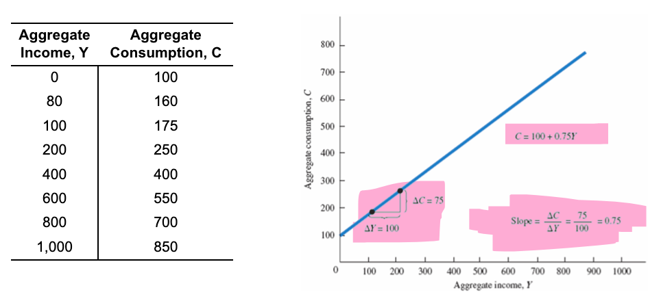
what is consumption at income of 0?

as incomes rises…

for every ___ increase in income, consumption rises by ___

slope of line is ___

DERIVE SAVINGS FUNCTION:

In this simple consumption function, consumption is 100 at an income of zero.​

As income rises, so does consumption. ​

For every 100 increase in income, consumption rises by 75.

The slope of the line is 0.75

S = -100 + 0.25Yd

savings function

Y_d = C + S

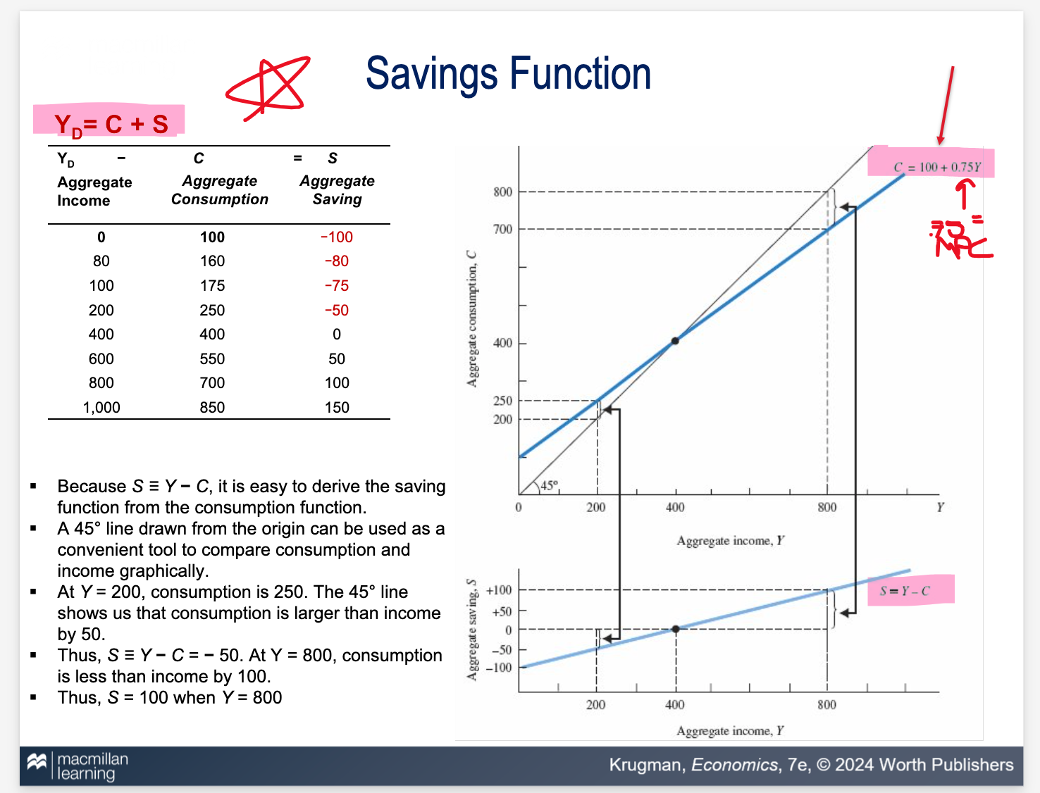
📊 Savings Function in Economics

• What does the graph show about income, consumption, and savings?

✅ Key Concepts:

• The savings function is derived from the consumption function:
  YD = C+S (Disposable Income = Consumption + Savings)

• Consumption Function: C=100+0.75Y

  • MPC=0.75MPC (Marginal Propensity to Consume)

• Savings Function: S = Y − C

  • When income is low, savings are negative (dissaving).

  • When income increases, savings become positive.

📈 Graph Interpretation:

• The 45° line represents when income = consumption.

• If a point is above the line, there is dissaving (spending more than earning).

• If a point is below the line, there is positive saving (income exceeds consumption).

• Example: At Y = 200, C= 250 → Saving is -50 (dissaving).

• At Y = 800. C = 700 → Saving is 100 (positive saving).

assessment #4:

Assume there are no taxes. The equation for the consumption function is given to​ be:​

​

C​ = 150​+ 0.60YD, Where Y represents aggregate income.​

​

Determine the equation for the saving​ function:​

s = -150 + 0.4Yd​

What does stagnation refer to in economics?

A period of little or no growth in GDP, often accompanied by high inflation and low demand.

How does consumption compare to investment in terms of volatility?

Consumption tends to be more stable and less volatile than investment, which can fluctuate significantly based on economic conditions.

What is cost-push inflation?

Inflation that occurs when the costs of production increase, leading businesses to raise prices to maintain profit margins.

What are common causes of cost-push inflation?

Increases in the prices of raw materials, labor, or other production inputs that raise overall production costs.

planned investment spending

the investment spending that businesses intend to undertake during a given period.​

depends on:

• interest rate

• expected future real GDP

• current level of production capacity

accelerator principle

• higher rate of growth in real GDP; higher planned investment spending

• lower growth rate of real GDP; lower planned investment spending

• production capacity

  • operating at full capacity; investments rise

inventories

stocks of goods held to satisfy future sales

unplanned inventory assessment

unexpected changes in inventories that occur when actual sales are more/less than businesses expected

Actual investment spending & formula

amount of money that businesses spend on new capital assets during a specific period of time

• I = I_unplanned + I_planned

assessment:

Suppose that in the year​ 2015, Oceanaire, Inc. produced 500,000 units of its lightweight scuba tanks. Of the 500,000 .it planned to​ produce, a total of 30,000 units would be added to the inventory at its new plant in Arizona. Also assume that these units have been selling at a price of $ 225 each and that the price has been constant over time. Suppose further that this year the firm built a new plant for $ 5million and acquired $ 3.5 million worth of equipment. It had no other investment​ projects, and to avoid​ complications, assume no depreciation.  ​

Now suppose that at the end of the​ year, Oceanaire had produced 500,000 units but had only sold 450,000 units and that inventories now contained 50,000 units more than they had at the beginning of the year. At $ 225 ​each, that means that the firm added $ 11,250,000 in new inventory.​

Oceanaire planned to invest ​?​

This year Oceanaire actually invested ?​

Next year Oceanaire should produce more or less? ​​

planned investment:

50000000 (new plant) + 3500000 (equipment) + (225*30000) = 1525000

Actual:

5000000 (new plant) + 3500000 (equipment) + (225*50000) = 19750000

PRODUCE LESS

• actual would decrease production

Let’s assume that there are no taxes (T=0) or transfers and no International market. Hence no (G) + (Xn).

& assume I_planned is fixed, so​ …

GDP = C + I

Y_d = GDP​

AE_Planned = C + I_planned = GDP​

Fundamental in Keynesian economics; illustrates the relationship between production and expenditure.

Y = AE

Shows how consumption and investment contribute to total income.

Y = a + bYd + I

equilibrium is when

I_unplanned = 0

Suppose the level of planned aggregate expenditure in an economy is $500 and real GDP is $600. According to our model (multiple choice:​

1. unplanned increases in inventories are occurring.​

2. unplanned decreases in inventories are occurring.​

3. inventories will be unaffected and will remain at the planned inventory level.​

4. excess production will continue, since there is no mechanism to restore the level of production to the level of spending.​

unplanned increases in inventories are occurring.​

if GDP (Y) > AE_planned ; then…

if GDP (Y) < AE_planned ; then…

I_unplanned is positive

I_unplanned is negative

2 possible sources of a shift of the planned aggregate spending line:​

a change in I_planned

shift of CF (aggregate consumption function)

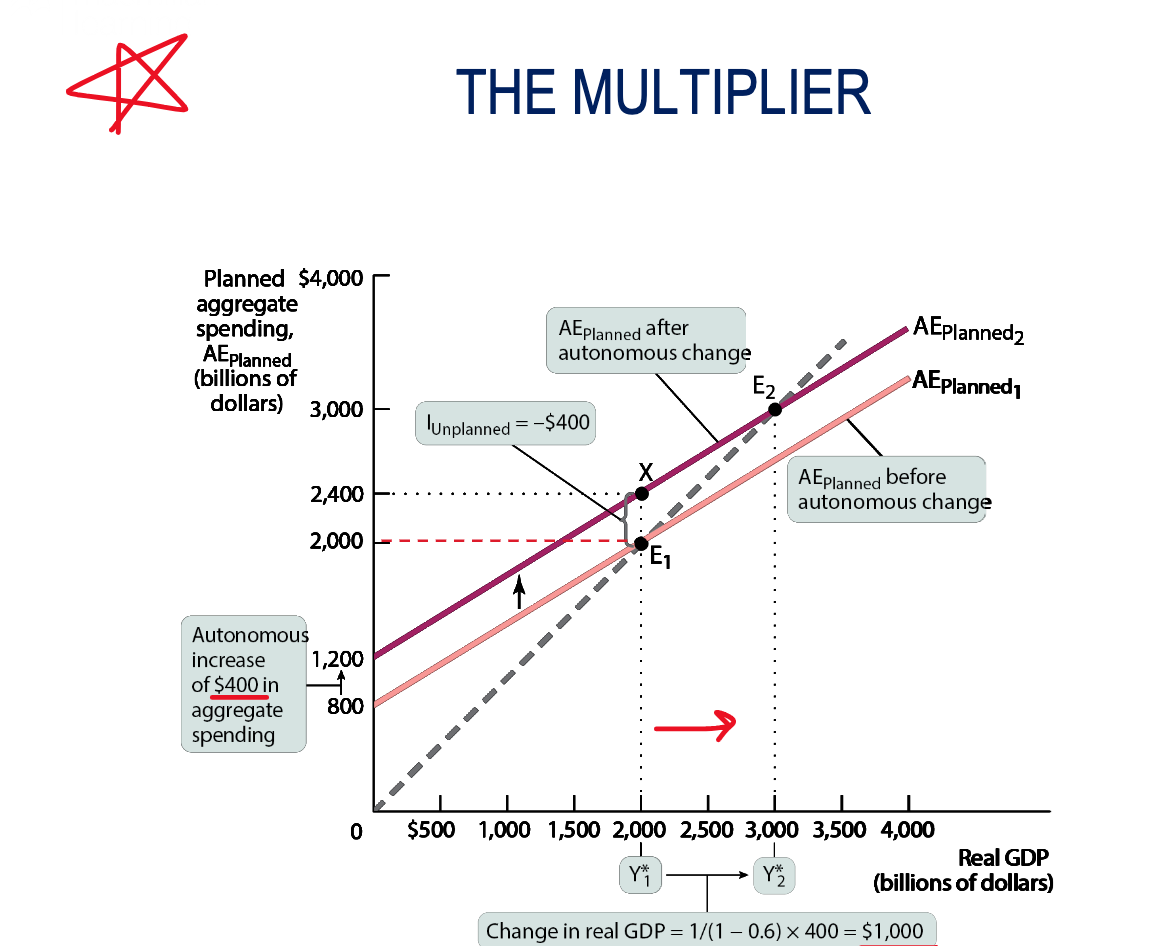
using the image, calculate the multiplier

Given: MPC = 0.6; real GDP increases by 400

1 / (1-MPC)

If an autonomous spending increase of $400 leads to a total GDP change of $1,000, the multiplier is:

(3000-2000) / (1200-400) = 2.5

Setting it equal to the multiplier formula:

1 / (1−MPC) = 2.5

Solving for MPC:

MPC = 0.6

multiplier effect

A change in spending (like a drop in investment) leads to a larger overall change in GDP.

• ex. businesses cut spending by $100 million, the economy might shrink by $300 million due to reduced consumer spending and income; everyone can end up worse off due to job losses and less money in the economy.