PSYC 359: Advanced Research Methods

statistical inference

specified null that is tested with set significance criterion - based on assumption null is true

4 components of inference

1. sample size (n)

2. significance criterion (α)

3. Statistical power (1 - β)

4. Effect size (δ or p)

   If you have ¾ you can determine the 4th

type I error (α)

rejecting a null hypothesis when it is actually true - when null is true, for alpha = 0.05 there is a 5% chance of error

type II error (β)

retaining a null when it is actually true - if null is false, β x 100% of the time we make a Type II error

statistical power

probability of correctly rejecting a false null (1 - β)

type S error

rejecting a false null, but getting the direction of the relationship wrong (only for one-tailed tests)

type M error

error in estimation of magnitude of the effect (getting effect size wrong)

type IV error

an incorrect interpretation of a correctly rejected null

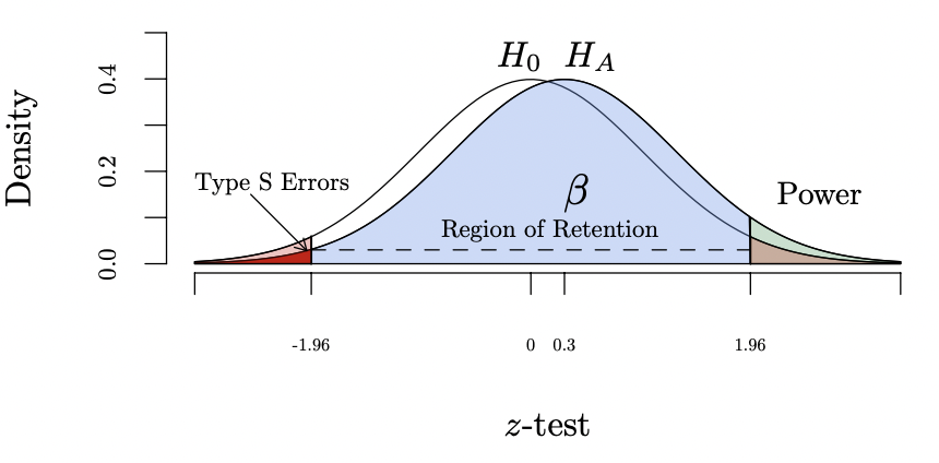
statistical power and inferential errors graphed

• type I error = light red region on H0 distribution

• type II error = blue part of HA distribution in region of retention

• type s error = dark red region in HA distribution below -1.96

if i retain the null, what is the probability that i have made a Type I error?

0% - can’t make a type I error

if i reject the null, what is the probability that i made a Type I error?

0 or 1 - either didn’t or did make a Type I error

if i reject the null, what is the probability that I made a Type II error?

0% - can’t make a type II error

if the null is false in reality, what proportion of 1000 researchers examining this hypotheses with make a Type I error?

a (usually 5%)

sampling distribution

distribution of a statistic calculated from all possible distinct random samples of of same size n drawn from population

expected value

mean of sampling distribution

standard error

standard deviation of sampling distribution

central limit theorem (CLT)

know mean, standard deviation, form of sample distribution of sample means for the sample distribution of the sample mean when when it is not possible to take all possible samples

mean of sampling distribution of sample means

E(x̄) = μ (equal to population mean)

standard deviation of sample means

standard error of the mean (σx̄ ̄ = σ/√n)

• n = sample size for mean

• σ = standard deviation for population

direct route hypothesis testing

compute parameters of interest on entire population using descriptive statistics (never know parameters of entire population)

indirect route hypothesis testing

compute descriptive statistics on random sample from population and infer values of population parameters and draw conclusions

scientific hypothesis

relationship/effect researcher expects to find - restated into null and alt hypotheses for indirect testing (mutually exclusive and exhaustive together)

null hypothesis (H0)

involves a prediction about exact value of population parameter - assumed to be true

• always contains an equity symbol ≤, ≥, or =

• H0 :μ = 120, H0: μ ≤ 100, H0 : σ = 11, H0 : μ1 − μ2 = 0

alternative hypothesis (HA)

accepted if H0 is rejected

• always contains and inequality symbol: <, >, or ̸=

• HA :μ < 120, HA : σ ̸= 11

8 steps of hypothesis testing

1. state problem and nature of data (nature = nominal, ordinal, interval, ratio, censored, truncated)

2. specify and state hypothesis to be tested (scientific, null, alt)

3. draw random sample of size n from population (randomly selected and representative)

4. determine sampling distribution of statistic being calculated (mean, SE, form of null distribution)

5. specify level of significance

6. determine regions of retention and rejection

7. calculate value of statistic of interest

8. test hypothesis and reject the null if it falls in region of rejection or retain the null if it falls in region of retention

p-value

probability of observed data or more extreme under the null sampling distribution

• doesn’t tell us the probability of the null (effect size)

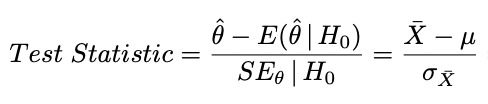
test statistic

general formula simply number of standard errors from the null sampling distribution

• based on theoretical sampling distribution of null

• use common reference distributions (z, t, etc.) to determine probabilities of the data

• θ is the population parameter of interest

• estimated by statistic θˆ

• E(θˆ| H0) is the expected mean of null sampling distribution for the statistic.

• SEθ | H0 is standard error for the statistic when null is true.

central distributions

distribution of test statistic under the null of no effect

• λ = 0 - all you require are central distributions

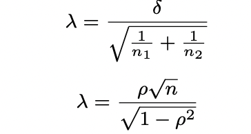
non-centrality parameter (λ)

measure of the degree to which a null hypothesis is false

• forms confidence intervals for effect sizes

• function of population effect size and sample size

probability function

used to obtain p-value - probability of a specific value and lower or higher

• given the quantile, calculate the probability

quantile function

determine test statistic that has specified probability of occurring

• given the probability, calculate the quantile

• for two-tailed tests (normal and t-distributions), divide alpha by 2

critical values

quantiles on Ho distribution

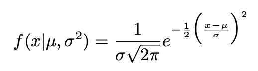
normal distribution

• population mean μ

• variance σ2

Gauss’s 3 assumptions for normal distributions

1. small errors more likely than large errors

2. for any error ε, likelihood of ε is same as that of −ε

3. with several measurements containing independent errors, average has highest likelihood of producing observed data (max likelihood estimate of underlying parameter)

probability calculation for normal distribution

pnorm( )

• calculate 2-tailed tests: 2 * pnorm( )

quantile calculation for normal distribution

qnorm( )

chi-square χ2(df)- distribution

sample distribution of sample variation - Function of squared normal distribution

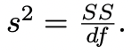
• each df represents another independent observation from normal distribution

• sample variance is a function of since variance is a squared value when original observations are normally distributed

• mean of sampling distribution is its df

probabilities for chi-squared distributions

pchisq(critical value, df, lower.tail)

• all p-values inherently two-tailed (don’t divide a)

quantiles for chi-squared distributions

qchisq(alpha, df, lower.tail)

• not divided by 2

degrees of freedom

finite sample size correction - account for variance in sample

assumptions of chi-squared distributions

• residuals are independent: we have correct df - violating has huge impact on type I error

• normally distributed: if violated, we don’t know distribution of sample variance

• estimation of sample variation gets better as sample size increases

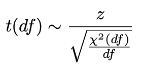
t-distribution (student’s t-test)

ratio of normal distribution and square root of chi-square distribution

• statistic in denominator instead of a parameter

• standard deviation is a function of sqrt(χ2(df))

probabilities for t-distribution

pt(critical value, df, lower.tail)

• 2x when wanting to find both tails

quantiles for t-distributions

qt(alpha, df, lower.tail)

• divide alpha by 2

F-distribution

ratio of 2 variance estimates, ratio of χ2 (df ) variables

• has 2 df associated with it

• commonly used in context of ANOVA

• always two-tailed

• when df1 = 1, it is the square of t-distribution

• when df2 = infinity, it is the chi-squared distribution/df

probabilities for F-distribution

pf(critical value, df1, df2, lower.tail)

quantiles for F-distribution

qf(a, df1, df2, lower.tail)

• a not divided by 2

Which statistic has a lower p-value z = 2.0 t(16) = 2.0?

z = 2.0

which test statistics have the same p-values? z = 2.0, t(16) = 2.0, χ2(1) = 4.0 F(1,16) = 4.0?

t and F, z and χ2

why does pnorm(2.00, lower.tail=FALSE) not give us the p-value 4.0 but pchisq(4.0, df=1, lower.tail=FALSE) does?

is inherently two-tailed but normal distributions aren’t, so to get that value, you would have to multiply it by 2

for a = .05 under normal distribution, is critical value of 1.96 (a) a p-value, (b) a quantile, (c ) a parameter, or (d) a test-statistic?

quantile

what do df for a t-test indicate? does this tell us about the amount of info in the means or variance?

Inform us about amount of information (and thus precision) associated with estimate of variance that is being used incomputing the t-test

which statistic’s sampling distribution is the χ2(df)-distribution related to?

sampling distribution of the sample variance0

scatterplot

graph where each individual data is represented by a plot on the graph - use jitter and loess curve to improve its utility

jitter

small amounts of random noise in x or y-axis to avoid overplotting

loess curve

nonparametric smoother (doesn’t presume any relation between the variables)

• control span (amount of smoothing) and fitting model (relationship you want to use to estimate relationship within each span)

• simply estimates a relationship based on observed data

• more properly approximated observed data

pearson product-moment correlation (r )

measure of linear association between two variables after removing units from each variable by standardizing them

• common effect size measure

• formula provides correlation for other methods

• presumes linearity and independence, normality, homogeneity of variance

• attenuated by restricting range on observed variables (reduces SD and reduces the magnitude)

• based on t(df) distribution - df = n-2

spearmen correlation (rs)

association between ranks of two variables - replace each observed value for x and y with its rank

• more robust to assumption of normality, but statistical power is reduced

• useful for monotonic relationships (association is strictly increasing or decreasing)

point biserial correlation (rpb)

pearson correlation between a dichotomous variable (like treatment/control) and a continuous measure

• just use Pearson to compute - for distinguishing one of the variable is dichotomous

• based on t(df) distribution - df = n-2

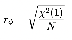
φ correlation

measure of association between two dichotomous variables

• done using Pearson r formula if data are numeric or using cell counts in a table

• table: define each cell and then calculate - 2×2 table = A, B, C, D

dichotomous

a classification system that divides things into two mutually exclusive categories.

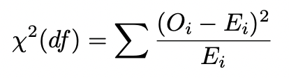
χ2(df)-test for independence

tests difference between what we expect to see under null of no association vs observed data

• significant = rejection of null

• function of observed count (O) and expected count (E) for cell i as follows where df = (#rows - 1)(#columns - 1)

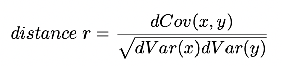
distance correlation (dr)

measures dependence between x and y by computing distance of each observation from every other observation

• addresses issues in Pearson correlation insensitive to deviations from linearity

• 0 to 1 (0 = complete independence, 1 = perfect dependence)

• dcor.ttest(x, y) in R

• probability under the null using a large number of random correlations - dcor.test(x, y, R=10000)

• unbiased dr is smaller than r

do multiple studies in an article safeguard inferences?

No

• under standard data-analytic and research practices make significant results easy to obtain (omitting variables of no significance)

familywise type I error rate

probability of at least 1 type I error being. made across set of tests in a manuscript

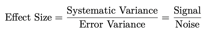
effect size

degree to which treatment changes the treated subjects relative to control subjects/degree to which phenomenon is or isn’t present in the population'

• ratio of systematic variance relative to error or residual variance - signal-to-noise ratio

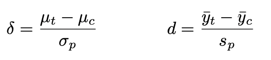
effect size: Cohen’s d

standardized mean difference - difference between treatment and control mean relative to standard deviation

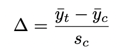
glass’ ∆

measure of effect size

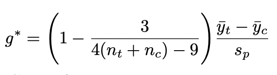
Hedges’ g

unbiased estimate of standardized mean difference based on pooled standard deviation

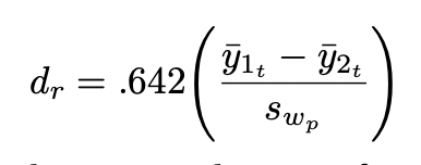
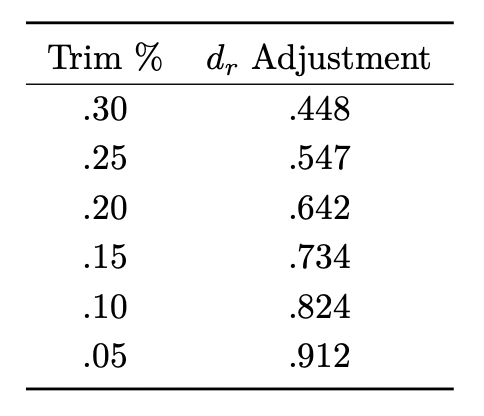
standardized mean difference for robust t-test (dr)

y1 and y2 = trimmed means from groups 1 and 2

swp = pooled Winsorized standard deviation (.642 adjustment for 20% of each tail)

statistical power

probability of correctly rejecting a false null

• function of sample size, alpha, and effect size

determining statistical power for one-sample z-test

1. Draw null hypothesis theoretical sampling distribution.

2. Calculate regions of retention and rejection.

3. Determine and draw alternative hypothesis theoretical sampling distribution on the same graph.

4. Calculate power as proportion of sample means in alternative hypothesis sampling distribution that is region of rejection.

determining statistical power for independent sample t-tests

same as z-test, except:

• can’t express hypothesis distributions and regions in terms of specific scores as we don’t know population parameters

• indicate ncp when calculating pt( ) (treatment mean - control mean / standard deviation

if effect size and alpha remain same, what happens to power when n increases?

it increases

if you decrease effect size, why does power decrease?

mean z-test under HA decreases as a result which reduces power

how are beta and power related

power = 1 - beta

if you increase alpha from .05 to .10, what happens to power?

it increases because increasing alpha also increases the region of rejection

For independent samples t-test, if effect size and α remain the same, and n increases, there are two reasons statistical power increases. What are these two reasons?

1. noncentrality parameter (mean of the alt distribution on the t-test scale) increases.

2. critical t-value decreases, which increases region of rejection

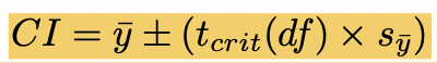
confidence interval

index of uncertainty associated with a statistic (usually 95% for alpha = .05)

• calculated by hand once critical t-values are determined

• tcrit tells how far estimates are from true population through number of standard errors from 0

• intervals will cover population mean difference in 95% of random samples

confidence intervals for single means

one sample size

standard error of the mean (sy ̄)

standard deviation / sqrt(n)

confidence interval for mean differences

2 sample sizes and 2 means

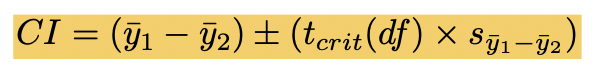
sy1 - y2

estimated standard error of difference between 2 means

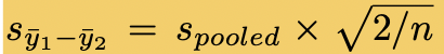
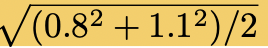
spooled

pooled standard deviation between 2 means

• sqrt((var1² + var2²)/2)x

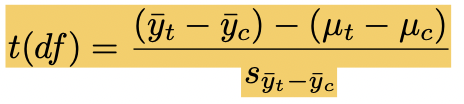
p-value for difference between two means

differences between sample variances - null hypothesis / SE between means

• μt − μc = null (often = 0)

calculating CIs for standardized effect size estimates

function of population parameter and where it intersects with observed statistic

• not calculable unless we assume normality and homogeneity for errors, so resampling approximates these CIs

• values of that have cumulative probabilities between .975 and .025