Applied Econometrics

Time Series

Sequence of observations taken sequentially in time

Lag Operator

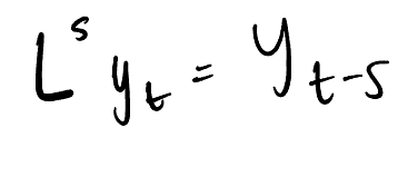
What does the difference operator express

Differences between consecutive observations of a time series

Define a Univariate Time Series Analysis (and what process it is)

Single time series.

Stochastic Process

Purpose of univariate time series (2)

• Develop models/methods that best describe an observed time series

• forecasting

Define

Multivariate Time Series Analysis

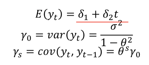
A time series is stationary if (3)

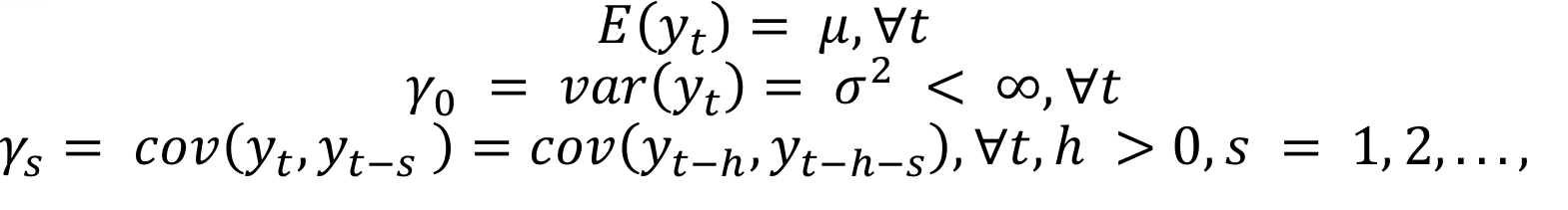
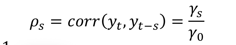
Autocorrelation coefficient

How does p_s behave in a stationary process

• Time constant

• Decreases quickly to 0, as the lag length increases

Shocks to a stationary process are (2)

• temporary

• short memory

What is Non-stationary Process

• non mean reverting

• Exhibits trends

Why is non-stationary not efficient (4)

• empirical results from one period cannot be generalised to other periods

• Forecasting is meaningless

• The series cannot be easily modelled

• Spurious regression

What is a WN process

Sequence of uncorrelated random variables with a constant mean and constant variance . It has no memory.

White Noise Properties

If time series is WN, the sample autocorrelations will

Approx equal to zero

Purpose of ARCH family of models

Models that are capable of dealing with the volatility of series

ARCH model suggests…

Variance of the residuals at time t, depends on the squared error terms from past periods

So it is better to model the mean and variance

Format of ARCH Model

Property of ARCH

Variance depends on one lagged period of the squared error terms

Steps to Identify ARCH model

1. Estimate by OLS and obtain residuals

2. Regress the squared residuals to a constant and lagged squared residuals

3. Compute the LM = (n-p)R² statistic and compared with critical values

4. Conclude

What is the GARCH model

Includes the lagged conditions variance terms as autoregressive terms

Format if GARCH model

Identify GARCH model

Maximum likelihood estimator

What is a TGARCH model

Adds dummy into variance equation to test whether is a statistically significant difference when shocks are negative

Format of TGARCH

Format a Autoregressive Model

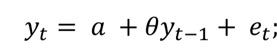
Statistical Properties of AR model

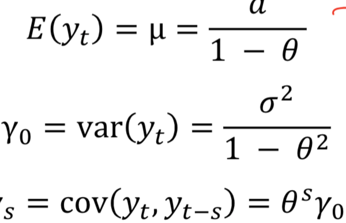
Autocorrelations of AR models..

Decay quickly as lag length increases

Check for Stationarity in AR model

1. Replace L by z in AR lag polynomial and set equal to zero (characteristic equation)

2. If roots of z are greater than than 1 in absolute value = stationary

AR to MA

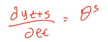
Impulse Response of AR

Format the Moving Average Model

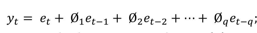
Statistical Properties of MA model

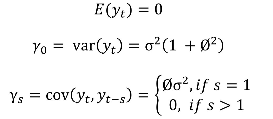
Autocorrelations of MA models…

Decay quickly towards zero as lag length increases

Steps to check invertibility (MA)

1. Set z = L in the MA lag polynomial, and set equal to zero (characteristic equation )

2. If all roots greater than 1 = it is invertinle

MA to AR

1. Solve model with respect to et

2. Rearrange for Yt in LHS

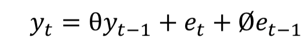
Format the Autoregressive Moving Average Model

Check for stationarity ARMA

1. Replace L by z in the AR lag polynomial of order p, ant set equyal to zero (characteristic equation)

2. If all roots greter than 1, it is stationary

ARMA to MA

Check for invertibility ARMA

1. Replace L by z in the MA lag polynomial and set equal to zero (characteristic equation)

2. If all roots are greater than 1 = invertible

What does the Box-Jenkins approach infer

Which stationary models has generated the stationary series

Box-Jenkins Steps

1. determine the order (p,q) using the information criteria

2. estimate parameters

3. Diagnostic testing ( resdiuals should behave like white noise)

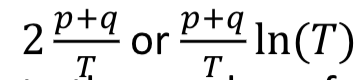
Order Identification Options

• Choose the maximum pmx and qmax

• Then estimate the Maximum likelihood for all combinations

  • Estimate using the AIC OR BIC

Problem of Adding Lags

Over parameterised models.

Can be rectified using a penalty term

What is a non-stationary series

A series containing a trend (dertministic or stochastic)

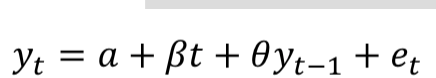
What is a trend stationary model

Trend stationary series with a determinist trend

Format a tren staionary AR model

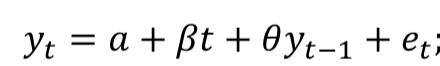
Properties of trend stationary AR

mean varies with time

Define de-trending

Process of removing a trend in a series

Steps to detrending

1. Estimate the OLS and obtain the residuals

2. Detrend the residuals

3. Apply the box-jenkins to the de-trended series

Define Stochastic Trend

Trend that evolves randomly over time (no steady trend direction)

Stochastic trend alternative names:

• Difference stationary series

• Intergrated series

• Unit root series

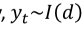
A stochastic trend series that contains 𝑑 ≥ 0 unit roots is..

1. Intergrated of order d

   

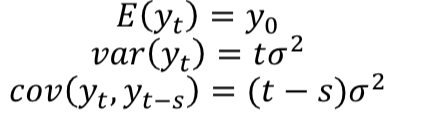
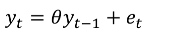
Format the Random Walk model

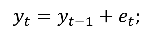
What is the RW model

• Stochastic trend model with one unit root

• Integrates of order one

Random walk statistical properties

IRF of RW

How to remove unit root

Differencing

Steps to differencing

b

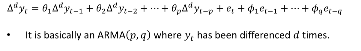
What is an ARIMA model

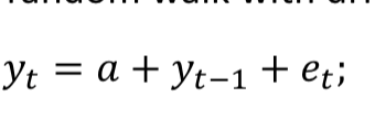
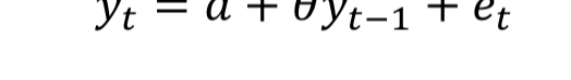
What is a random walk with drift model

Random walk model with an intercept

Format the RW model with drift

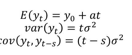
RW Model with drift Properties

DF test (clear trend direction)

1. inspect series

2. Set up

3. Test H0: unit root vs H1:

4. Rewrite the model in differenced form

5. Estimate using OLS

6. DF test

7. compared t to DF critical value

DF Test (no trend)

1. Inspect

2. set up

3. Difference the model

4. Estimate using OLS

5. DF test H0: unit root. H1: staionary

6. compared t to DF critical value

DF test (zero sample average)

1. Inspect

2. set up

   

3. Difference the model

4. Estimate using OLS

5. DF test H0: unit root. H1: stationary

6. compared t to DF critical value

DF test is valid if

et is a white noise process

Solutions to limitiation of DF

Augmented DF test; by adding lags of difference yt

ADF: Lag-length selection

1. Information criterion (AIC/BIC)

   1. estimate adf with lag lengths to max, including the difference yt

   2. Select with lowest AIC/BIC

2. General to specific

   1. Estimate the model with pmax lags

   2. check is resiuals are WN

   3. Test the last lag coefficient for significance

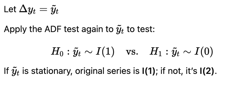
ADF fails to reject the null then..

Test for second unit root

Limitations of ADF ( and alternatives)

• ADF has low power (fail to detect stationarity)

• Alternatives:

  • DF-GLS (detrended ADF)

  • Philipps-peron

  • KPSS

What does a spurius regression result in

• OLS estimates are far away from zero.

• They are statistically significant.

• 𝑅sqaured is also relatively large

Finds a statistically significant relationship between uncorrelated variables due to unit roots

Correct spurious regressions by

Differencing and

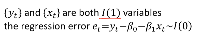
When is a series cointergrated

Test for Conintergration

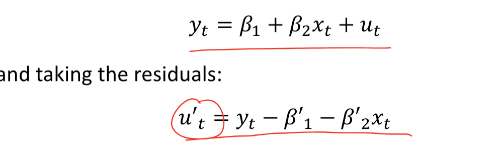
Engle granger test

• Make sure both xt and yt are I(1) then run the model with OLS

• apply DF (or ADF, or DF-GLSS etc) to obtained residuals

Why differencing successively to achieve stationarity is not ideal

1. We also difference the error process

2. No unique long run solution

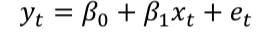
Find long run equilibrium of xt and yt (Co-intergration)

if ut ~ i(0) then the variables are cointergrated

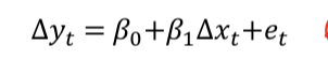
The Error Correction Model

Combines short and ong run information

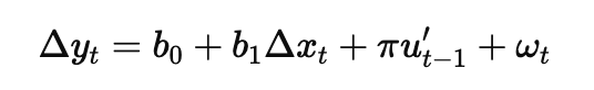
b1 - immediate effect of xt

pie - how much past period is corrected in t

Advantages of the ECM and Cointergration

• ECM measures how past imbalances are corrected over time

• by using first differences, ECM avoids spurious regressions

• ECM is easy to intergrate into general-to specific modellling

• error term is stationary, meaning there's an automatic mechanism that prevents long-run errors from growing indefinitely

Testing for Cointergration

Engle Granger Approach

1. test the variables for order of integration

2. estimate the long-run relationship and obtain the residuals

3. check for cointegration the order of integration of the residuals

4. estimate ECM

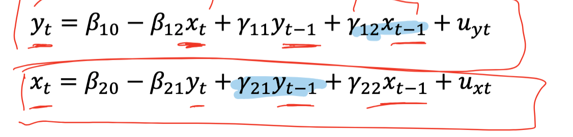
Vector Autoregression

time series 𝑦 that is affected by current and past values of 𝑥௧and, simultaneously, the time series 𝑥 to be a series that is affected bycurrent and past values of the 𝑦 series

Pros of VAR (3)

• Simple

• Estimation is simple

• VAR forecast are better compared to complex models

Cons of VAR (3)

• A-theoretic

• Loss of df

• Obtained coefficients are difficult to intepret

Test for VAR

Granger Causality

A variable 𝑦 is said to Granger-cause 𝑥, if 𝑥 can be predicted with greater accuracy by using past values of the 𝑦 variable rather than not using such past values, all other terms remaining unchanged.

VAR test results (4)

1. Lagged x statistically significant and y not. so x causes y

2. Lagged y statistically significant and x not. so y causes x

3. Both statistically significant = bi-directional causality

4. both no significant = indepoendent

Granger Causality steps

1. regress y on lagged y and obtain RSSr

2. regress y on lagged y and lagged x and obtain RSSu

3. H0: coefficients of lagged terms of x are equal to zero H1: coefficients of lagged terms X are NOT equal to zero

4. F- statistic and conlude

Define Probability of Success

Model the probability of choosing one of the alternatives

What is the base group

Alternative category that is not explicitly modelled

Why is OLS not suitable for modelling the probability of success

The dependent variable (response) is discrete but OLS treats as continous

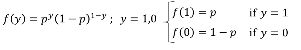
Y is said to have a bernoulli distribution with prob. mass function:

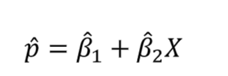
Format the linear probability model

• b2 is the change in the probability that is associated with a unit change in x

Limitations of LPM

• distribution of disturbance term consists of 2 specific values = binomial distribution = so standard errors are invalid

• Population variance of the disturbance tern is given byso

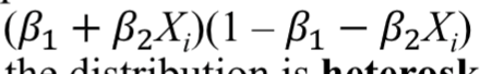
So it is heteroskedastic

• for alternative values of x, we can gain probabilities that are greater than 1etc

By OLS, the predicted probabilities are

How do we ensure predicted probabilitues are bounded by 0 and 1

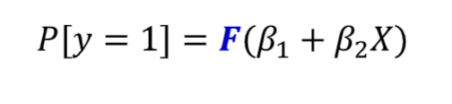
Ensure F is a probability distribution function. Standard normal cumulative distribution function and logistic distribution function

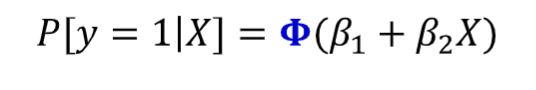
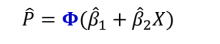
Format the Probit Model

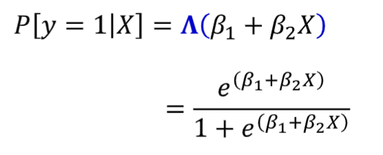
Format the Logit model

How do we obtain b1 and b2 from the logit/probit models?

The MLE chooses the parameter values that maximize the probability (or likelihood) of observing the sample actually obtained

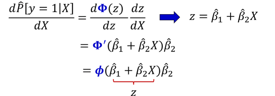
Predicted probability from Probit model

Format the Marginal effect of a one unit change in X (probit)