Quantitative Research Finals W3-W6

Skewness

• is a measure of asymmetry or distortion of symmetric distribution.

• it measures the deviation of the given distribution of a random variable from a symmetric distribution such as Normal Distribution.

Asymmetrical Distribution

• is a situation in which the values of variables occur at irregular frequencies and the mean, median, and mode occur at different points.

• If a distribution is not symmetrical or normal, it is skewed, i.e., the frequency distribution is skewed to the left or right.

Symmetrical Distribution

• occurs when the values of variables appear at regular frequencies and often the mean, median, and mode all occur at the same point.

• A distribution, or data set, is symmetric if it looks the same to the left and right of the center point may be either bell - shaped or U shaped.

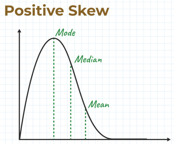
Right Skew

• Positive Skew

• L - shaped

• A right-skewed distribution is longer on the right side of its peak than on its left.

• means the tail on the right side of the distribution is longer. The mean and median will be greater than the mode.

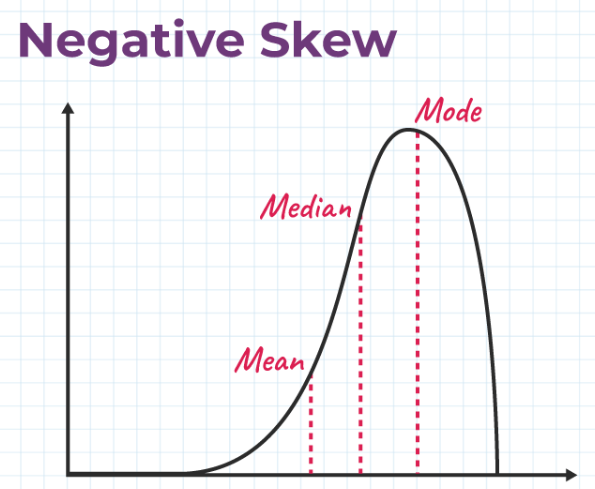
Left Skew

• Negative Skew

• J - shaped

• A left-skewed distribution is longer on the left side of its peak than on its right.

• means when the tail of the left side of the distribution is longer than the tail on the right side. The mean and median will be less than the mode.

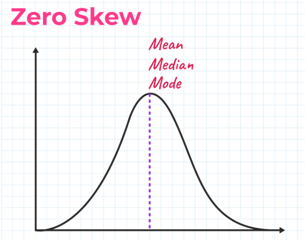
Zero Skew

• It is symmetrical and its left and right sides are mirror images.

Pearson’s first coefficients (mode Skewness):

• It is on the Mean, mode, and standard deviation.

• Use when a strong mode is exhibited by the sample data.

Pearson’s second coefficient (median skewness)

• It is on the distribution’s mean, median, and standard deviation.

• Use when data includes multiple modes or a weak mode.

Pearson Correlation

• The correlation coefficient is the measurement of the correlation between two variables.

• Pearson correlation formula is used to see how the two sets of data are co-related.

• The linear dependency between the data set is checked using the Pearson correlation coefficient.

• Also known as Pearson product-moment correlation coefficient.

• The value of the Pearson correlation coefficient product lies between -1 to +1.

• If the correlation coefficient iszero, then the data is said to be not related.

• A value of +1 indicates that the data are positively correlated.

• A value of -1 indicates a negative correlation.

Correlation

• is defined as the statistical association between two variables. A correlation exists between two variables when one of them is related to the other in some way. A scatterplot is the best place to start. A scatter plot (or scatter diagram) is a graph of the paired (x, y) sample data with a horizontal x-axis and a vertical y-axis. Each individual (x, y) pair is plotted as a single point.

Scatterplot

• can identify several different types of relationships between two variables.

  • A relationship has no correlation when the points on a scatter plot do not show any pattern.

  • A relationship is nonlinear when the points on a scatterplot follow a pattern but not a straight line.

  • A relationship is linear when the points on a scatterplot follow a somewhat straight-line pattern. This is the relationship that we will examine.

Linear Correlation Coefficient

• are used to measure how strong a relationship is between two variables.

• There are several types of correlation coefficient, but the most popular is Pearson’s. Pearson’s correlation (also called Pearson’s R) is a correlation coefficient commonly used in linear regression.

Pearson Correlation

• Correlation between sets of data is a measure of how well they are related. The most common measure of correlation in statistics is the _______. It shows the linear relationship between two sets of data.

• In simple terms, it answers the question, Can I draw a line graph to represent the data?

• Helps in knowing how strong the relationship between the two variables is. Not only the presence or the absence of the correlation between the two variables is indicated using the ___, but it also determines the exact extent to which those variables are correlated. Using this method, one can ascertain the direction of correlation i.e., whether the correlation between two variables is negative or positive.

Correlation coefficient of 1

• means that for every positive increase in one variable, there is a positive increase of a fixed proportion in the other. For example, shoe sizes go up in (almost) perfect correlation with foot length.

Correlation coefficient of -1

• means that for every positive increase in one variable, there is a negative decrease of a fixed proportion in the other. For example, the amount of gas in a tank decreases in (almost) perfect correlation with speed.

Correlation coefficient of 0 (zero)

• means that for every increase, there is no positive or negative increase. The two are not related.

Bowley Skewness

• is a way to figure out if you have a positively-skewed or negatively skewed distribution.

• very useful if you have extreme data values (outliers)or if you have anopen-ended distribution.

• is an absolute measure of skewness meaning that it is going to give you a result in the units that your distribution is in.

• could not be used to compare different distributions with different units.

• is based on the middle 50 percent of the observations in a data set. It leaves 25 percent of the observations in each tail of the distribution.

Open-ended Frequency Distribution

• one or more than one class is open-ended.

• It simply means that the lower limit of the first class is not given, or the upper limit of the last class is not given, or both are not given.

• It does not have a boundary.

Kelly’s Measure of Skewness

• is one of several ways to measure skewness in a data distribution.

• Kelly suggested that leaving out fifty percent of data to calculate skewness was too extreme.

• created a measure to find skewness with more data.

• Kelly’s measure is based on P90 (the 90th percentile) and P10 (the 10th percentile). Only twenty percent of observations (ten percent in each tail) are excluded from the measure.

Momental Skewness

• is one of four ways you can calculate the skew of a distribution.

• It’s called “Momental” because the first moment in statistics is the mean.

Kurtosis

• is a measure of whether the data are heavy-tailed or light-tailed relative to a normal distribution.

• Data sets with high kurtosis tend to have heavy tails, or outliers.

• Data sets with low kurtosis tend to have light tails, or lack of outliers.

• A uniform distribution would be the extreme case.

• describes the "fatness" of the tails found in probability distributions.

• Kurtosis risk is a measurement of how often an investment's price moves dramatically.

• A curve's kurtosis characteristic tells you how much kurtosis risk the investment you're evaluating has.

Yules Coefficient

• is used to measure the skewness of a frequency distribution. It takes into account the relative position of the quartiles with respect to the median and compares the spreading of the curve to the right and left of the median.

Categories of Kurtosis

1. mesokurtic (normal)

2. platykurtic (less than normal)

3. leptokurtic (more than normal)

Mesokurtic Distribution (Kurtosis = 3.0)

• This distribution has a kurtosis similar to that of the normal distribution, meaning the extreme value characteristic of the distribution is similar to that of a normal distribution.

• is a statistical term used to describe the outlier characteristic of a probability distribution that is close to zero.

Leptokurtic (Kurtosis > 3.0)

• excess positive kurtosis.

• appears as a curve one with long tails (outliers.)

• the "skinniness" of a leptokurtic distribution is a consequence of the outliers, which stretch the horizontal axis of the histogram graph, making the bulk of the data appear in a narrow ("skinny") vertical range.

• These have a greater likelihood of extreme events as compared to a normal distribution.

Platykurtic (Kurtosis < 3.0)

​

• have short tails or thinner tails than a normal distribution (fewer outliers.)​

• Refers to a statistical distribution with excess kurtosis value is negative.​

​

Normal Distribution

• also referred to as Gaussian or Gauss distribution, de Moivre distribution or bell curve.

• In a normal distribution, the mean is zero and the standard deviation is 1. It has zero skew and a kurtosis of 3.

• Are symmetrical, but not all symmetrical distributions are normal.

• The distribution is widely used in natural and social sciences.

• It is made relevant by the Central Limit Theorem, which states that the averages obtained from independent, identically distributed random variables tend to form normal distributions, regardless of the type of distributions they are sampled from.

Hypothesis Testing

• is also called significance testing

• refers to a statistical procedure used to assess the validity of a claim or hypothesis about a population parameter. Its purpose is to provide evidence that either supports or contradicts a stated belief or assumption.

• In research and data analysis it allows researchers to make data-driven decisions by evaluating hypotheses against available evidence.

4 Step Process

1. State the hypotheses.

2. Formulate an analysis plan, which outlines how the data will be evaluated.

3. Carry out the plan and analyze the sample data.

4. Analyze the results and either reject the null hypothesis, or state that the null hypothesis is plausible, given the data.

Null Hypothesis (Ho)

• represents the default position, asserting that there is no significant difference or relationship between variables Hypothesis (typically the null hypothesis says nothing new is happening) we try to gather to reject the null hypothesis.

Alternative Hypothesis (Ha)

• Also called research hypothesis

• Presents an alternative viewpoint, suggesting that there is indeed a significant difference or relationship. It represents the research hypothesis or the claim that the researcher wants to support through statistical analysis.