Hypothesis Testing

Hypothesis Testing

Uses sample data to make inferences about the population from which the sample was taken

• Assumes that the null hypothesis is true (if data is different from what is expected then null hypothesis rejected)

• it asks only whether the population parameter differs from a specific “null” expectation using probability

• basically put assumptions about a population parameter to the test

Ex: Instead of the estimation of how large is the effect it asks “Is there any effect at all?”

Making Statistical Hypotheses

Uses two clear hypotheses statements: the null hypothesis and the alternative hypothesis

• hypothesis about a population

Null Hypothesis (H0)

The default hypothesis, It is a specific claim about the value of a population parameter

• statement of equality where there is no difference, effect or chance (population parameter of interest is zero)

• Identifies one particular value for the parameter being studied

• Wants to be rejected to provide support for alternative research hypothesis

Alternative Hypothesis (HA or H1)

Includes every other possibility (parameter values) except for the one stated in the null;

• opposite of null and is nonspecific

• often the statement researcher hopes is true

Mutually Exclusive Hypothesis

One of the 2 hypotheses (alternative or null) is true and the other must be false

• analyze data to determine which is which

Two-Tailed (Non-Directional) Alternative Hypothesis (H1)

States that there IS an effect or difference but doesn’t specify the direction of the effect

• used when testing for any significant difference (increase or decrease)

• the significance level is divided between both tails of the distribution

One-Tailed (Directional) Alternative Hypothesis (H1)

States that there IS an effect and also specifies the DIRECTION of the effect

• used when testing for either an increase or decrease BUT NOT BOTH

• one-tailed: the new drug increase bp, or the new drug decreases bp

• the significance level is placed in one tail of the distribution

To reject or not to reject

Fail to reject the null hypothesis: means we technically “accept” the null hypothesis with data being consistent with it

Reject the null hypothesis: the data is inconsistent with the null hypothesis so reject it and support alternative hypothesis (H1)

Hypothesis Testing Steps

1. State the hypotheses

2. Compute the test statistic with the data

3. Determine the p-value

4. Draw the appropiate conclusion / make the decision of reject or fail to reject

Test Statistic

Number calculated from the data & is used to evaluate the results

• it is compared with what is expected under the null hypothesis

Null Distribution

The range of values that support the null hypothesis and assume it is true (not an exact value)

• we determine the sampling distribution of the test statistic by assuming that the null hypothesis is true

• the alpha value is both significance levels (the values that reject the null) added

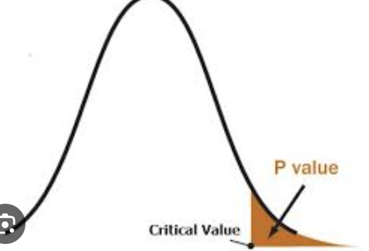
The P-value

The probability or likelihood of obtaining data more extreme/atypical than the data assuming the null hypothesis is true

• the probability of obtaining an extreme result

Small probability values (smaller p-value)

the null hypothesis is inconsistent with the data and we reject it in favor of the alternative hypothesis

• basically stronger evidence against the null hypothesis and we reject it

• HAPPENS WHEN P < .05

High probability values

Not enough evidence to reject the null hypothesis

• sample means close to H0 and states that the H0 (null) is true

Making A Decision

If the p-value is small, it lands in the critical region ( < 5%) causing a rejection of the null hypothesis (H0)

• the boundary is ( P < 0.05) to reject null = alpha level or level of significance ( α )

Null Distribution

Represents the distribution of a test statistic (e.g. mean difference, t-value, z-score) under the assumption that the null is true

• it is a bell-shaped curve (like standard normal distribution)

Confidence Interval (CI)

provides a range of plausible values for a population parameter (e.g., mean or proportion)

• typically constructed using sample data

Fail to Reject H0 with Confidence Interval (CI)

If it includes the null hypothesis value ( 0 for mean difference or 1 for odds ratio)

• the observed results isn’t significantly different from null expectation

Reject H0 with Confidence Interval (CI)

if the CI doesn’t include the null hypothesis

• suggests a statistically significant effect

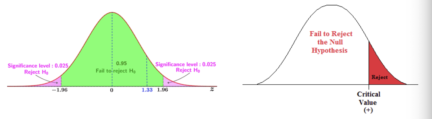
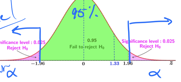
Graphical Interpretation

confidence interval of 95%

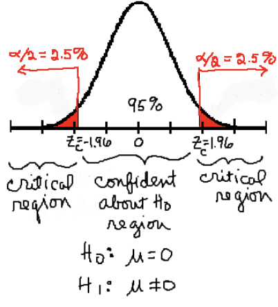
• for two tailed hypothesis test, the significance level (or α level) is at 0.05

• the critical values from the null distribution (both sides at + or - 1.96 z value) determine the cutoff pts for the CI & hypothesis test

Errors in Hypothesis Testing

Chance can affect samples & some uncertainty cant be quantified

• rejected the H0 doesn’t mean the null is false and failing to reject the null doesn’t mean it is true

• two types of errors: TYPE I ERRORS, AND TYPE II ERRORS

Critical Values

The cutoff pts from the null distribution that determine rejection regions based on the chosen significance level ( α )

• defines the rejection region for null hypthesis

  • if test statistic exceeds a critical value, H0 rejected

• Used to construct the Ci & determine the p-value threshold for significance

Type I Error

False Positive Probability = α

• Null hypothesis states to be true but it is actually rejected (false positive)

The incorrect rejection of a true null hypothesis

• alpha level tells the probability of committing a type I error (if alpha = 0.05 then we would mistakenly reject is 5% or 1/20)

Type II Error

False Negative Probability = β

• Null hypothesis stated to be false but it is actually not rejected (accepted)

Failing to reject a false null hypothsesis

• if a null is false we need to reject it

How to reduce type I error rate

By using a smaller alpha value

• has the side effect of increasing the chance of committing type II error

• reducing alpha makes the null more difficult to reject when true but also makes it more difficult to reject when false

False Positive (Type I Error)

Occurs when a test incorrectly indicates the presence of a condition when it is actually absent

• test incorrectly classifies a negative case as positive

Power

Probability found in Type II error that states random sample taken from a pop will, when analyzed, lead to rejection of a false null)

• quantified using alpha level, sample size, effect size, & the number of tails in a test

Power = 1 - β

False Negative (Type II error)

Occurs when a test fails to detect a condition that is actually present

• the test incorrectly classifies a positive case as negative

Sensitivity (True Positive Rate, Recall)

Measures the ability of a test to correctly identify those with the condition

• portion of actual positives that are correctly identified as positives

MEASURE OF TEST ACCURACY (TELLS HOW WELL A TEST DETECTS TRUE POS)

Higher Sensitivity

Fewer false negatives

• sensitivity tells how well the DS test detects DS when it is actually present

Recall

It measures how well the test recalls all true positive cases

• another term for sensitivity

Specificity (true negative rate)

Measures the ability of a test to correctly identify those without the condition

• portion of actual negatives correctly identified as negative

Higher Specificity

Fewer false positives

• tells how well the DS test avoids falsely diagnosing DS when it is actually absent

Statistical Power

Measures the probability of correctly rejecting a false null hypothesis

• power is the probability of avoiding a false neg

Ex: detecting an effect when one truly exists

Are sensitivity & power the same?

Conceptually similar (both measure the ability to detect a true pos) but applied in different contexts

• sensitivity used in diagnostic tests (medical testing, calssification problems)

• Power is used in hypothesis testing (experiments, stats studies)

They are the same in the context of diagnostic tests

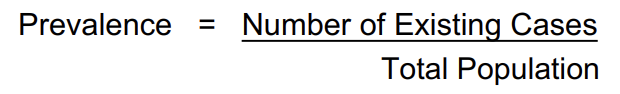
Prevalence

the portion of a population that has a specific condition or disease at a given time

• typically expressed as a percentage or as a fraction per 1000 or 100,000 people (depending on the context)

Ex: Prevalence of DS = 1 in 1000 pregnancies ( for every 1000 pregnancies, 1 has DS = 0.1%)

True Positive (TP)

Sensitivity x Total # of Cases

• the cases where the test correctly identifies DS

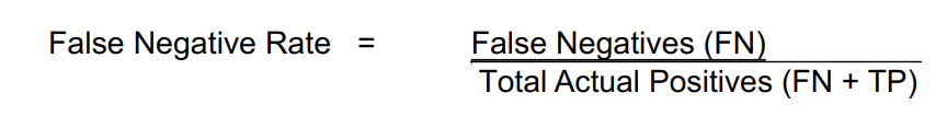
False Negatives (FN)

( 1 - Sensitivity) x Total # of Cases

• cases where the test fails to detect DS

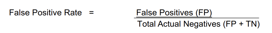
False Positive (FP)

False Positive Rate x Total Non # of a Certain Case

• ex: Total non-DS cases = 999,000 if 1 in every 100,000 children born has DS

• Cases where the test incorrectly identifies a normal pregnancy as having DS

True Negatives (TN)

(1 - False Positive Rate) x Total Non-DS Cases

• the cases where the test correctly identifies a normal pregnancy

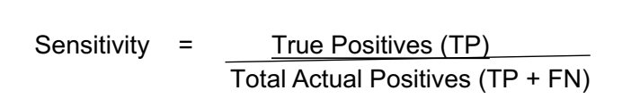
Sensitivity (True Positive Rate)

Tells how well the test detects DS when it is actually present

Sensitivity = TP / Total Actual Positives (TP + FN)

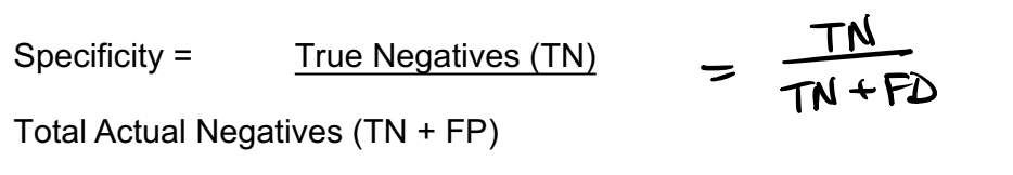
Specificity (True Negative Rate)

Tells how well the test correctly identifies pregnancies that DO NOT have

Specificity = TN / TN + FD

Power in diagnostic testing

Power is Equivalent to sensitivity because it represents the ability of the test to detect a true condition

• power = sensitivity in diagnostic testing (LIKE DS)

Goodness-of-fit Test

Method for comparing an observed frequency distribution w/ the frequency distribution that would be expected under a simple probability model governing the occurrence of diff outcomes

• statistical test to determine if sample data is accurate or skewed

• Compares observed data to expected data

Chi-Square goodness of fit test

used to determine whether a categorical variable follows a hypothesized distribution

• observed frequencies vs expected frequencies of a categorical variable

Expected Frequencies

Expected proportion * N

• sum of the expected values should be the same as the sum of the observed values (given rounding error)

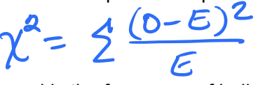
Chi-square (χ^2) test statistic

Measures the discrepancy btwn the observed & expected frequencies

• Observed = frequency of individuals observed in the __th category

• Expected = frequency expected in that category under the null

• Numerator = difference btw the data & what was expected

WHEN THE DATA PERFECTLY MATCHES EXPECTATIONS OF THE NULL THEN THE X2 VALUE IS ZERO

• any deviation leads to x2 > 0

• x2 uses absolute frequencies for observed & expected NOT the proportions of relative frequencies

The Chi-square distribution

It is a right-skewed distribution that allows only non-neg values

• has large counts condition (at least 5)

• It is a family of density curves

• The distribution is specified by its degrees of freedom (df)

Chi-square degrees of freedom = # of categories - 1

Assumptions of the x2 goodness-of-fit test

assumes that the individuals in the data set are a random sample from the whole pop

• each individual was chosen independently of all others & each member of the pop was equally likely to be selected for the sample

x2 statistic distribution

Follows a x2 distribution only approximatley

• should have an expected frequency less than 5

• no more than 20% of the categories should have expected frequencies les than 5

IF CONDITIONS NOT MET, TEST BECOMES UNRELIABLE

Degrees of freedom

Based on which analysis being conducted

• # of independent pieces of info used to calculate a statistic

approximates the null hypothesis of independence

• calculated by counting the (number of rows - 1) times (the number of columns - 1)

Chi-square contingency test

Displays how the frequencies of diff values for one variable depend on the value of another variable when both are categorical

• determines whether, & to what degree, 2 or more categorical variables are associated

Helps decide whether the proportion of individuals falling into diff categories of a response variable differs among groups

DETERMINES WHETHER THERE IS A STATISTICALLY SIG DIFF BTWN EXPECTED FREQ & OBSERVED FREQ IN 1 OR MORE CATEGORIES OF A CONTINGENCY TABLE

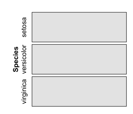
Mosaic Plot

Visualize data from 2 or more qualitative variables

• represented as rectangular areas

• represents the relationship between two variables

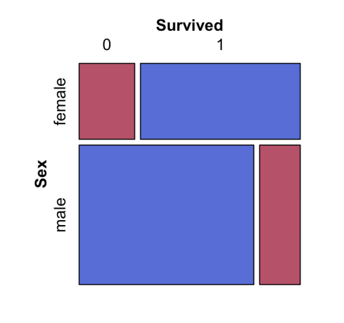
Independent Relationship Mosaic Plot

If the relationship btwn 2 variables is independent the bars would be equal in area

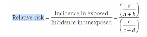
Estimating Association in 2 × 2 Tables: Relative risk

Relative risk is used to measure the association between an exposure & an outcome

• calculated as the ratio of the probability of the outcome in the exposed group to the probability in the unexposed group

Relative risk is the probability of the undesired outcome in the first group / the probability in the other desired group

Relative Risk (RR) = 1

RR = 1, risk in exposed is equal to risk in unexposed (no association)

• the null value for relative risk = indicates no difference between the groups

Relative Risk (RR) > 1

risk in exposed is greater than risk in unexposed (positive association, possibly casual)

Relative Risk (RR) < 1

risk in exposed less than risk in unexposed (negative association, possible protective)

Null value for risk difference

Is 0

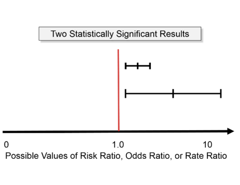
CI doesn’t contain the Null value (RR = 1)

Can say the finding is statistically significant

• if RR does not = 1 then findings are statistically significant (unlikely to have occurred by chance)

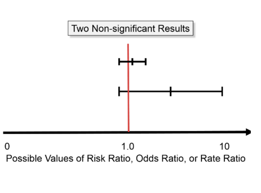
CI for the relative risk includes null vaue of 1 (RR = 1)

There isn’t sufficient evidence to conclude that the groups are statistically significantly different

• If RR = 1 then the findings are not statistically significant (occurred by chance)

Reduction in Relative Risk (RR)

1 - RR ( 1 minus Relative Risk)

• expresses the risk ratio as a percentage reduction

• the difference in risk btwn the 2 groups w/ respect to the control group

The percentage decrease in risk caused by an intervention compared to a control group who didn’t have intervention

Reduction in Absolute Risk (ARR)

The risk in the control group minus the risk in the treatment group

• actual difference in risk between the treated & the control group

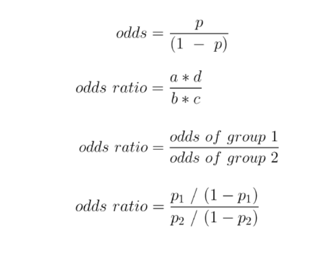
Estimating Association in 2 x 2 tables: the odds ratio

Odds ratio measures the magnitude of association btwn 2 categorical variables when each variable only has 2 categories

• one variable is the response variable (success & failure)

• Second variable is the explanatory variable (idenitfies the 2 groups whose probability of success is being compared)

Compares the proportion of successes & failures btwn the 2 groups

Focal outcome

The primary or main outcome variable of interest in a study

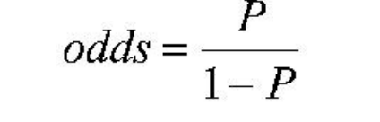
Odds

The probability of success or failure where success refers to the focal outcome

• The probability of success is p, probability of failure is 1 = p

If Odds = 1 (1:1)

One success occurs for every failure

Odds = 1 (10:1)

10 trials result in success for every one that results in failure

Odds ratio

The ratio of the odds of success btwn the 2 groups

Odds ratio = 1

The exposure is NOT ASSOCIATED with the disease

Odds ratio > 1

The exposure may be A RISK FACTOR for the disease

Odds ratio < 1

The exposure may be PROTECTIVE against the disease

Odds ratio vs Relative Risk

RR is more intuitive than OR as it is the ratio of proportions

• the values for the OR and RR will be similar whenever the focal outcome (outcome of the main variable) is rare

Odds Ratio Advantage

Can be applied to data from case control studies

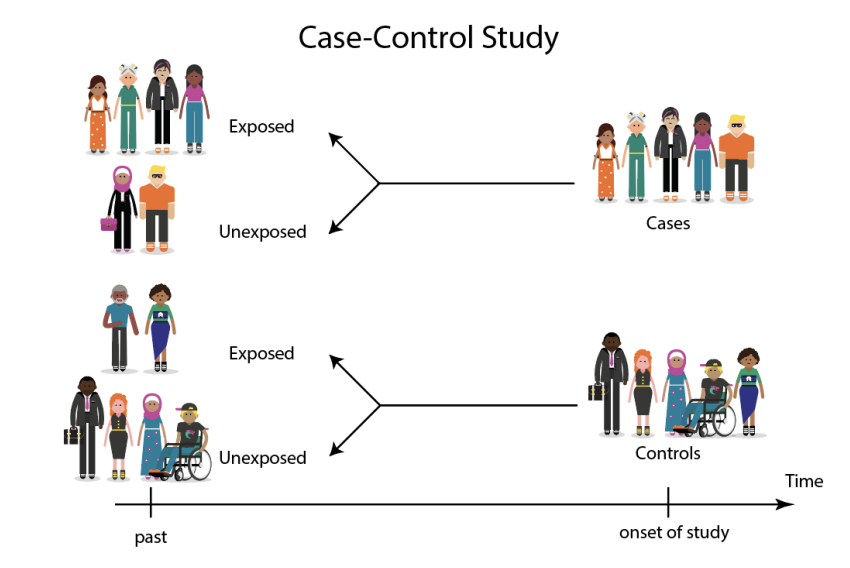
Case Control study

method of observational study where a sample of individuals having a disease or other focal condition (cases) is compared to a second sample of individuals who don’t have the condition (controls)

• the samples are otherwise similar in other characteristics that might also influence the results

The total # of cases & controls in the samples are chosen by the experimenter not by sampling at random in the pop

Chi-square contingency test

RR and OR allow to estimate the magnitude of association btwn 2 categorical variables

• doesn’t allow us to directly test whether an association may be caused by chance alone

Used as a test of association btwn 2 categorical variables

• tests the goodness of fit to the data of the null model of independence of variables

H0 on categorical variables

states that the categorical variables are INDEPENDENT

• means the probability of one occurring is equal to the probability of one occurring times the probability of the other event occuring

H1, OR H1 on categorical variables

states the categorical variables are NOT INDEPENDENT

Fischer’s Exact Test

Provides an exact p-value for an estimate of association in a 2 × 2 contingency table

• determines if there is a sig difference btwn 2 groups