Biostatistics Open Questions

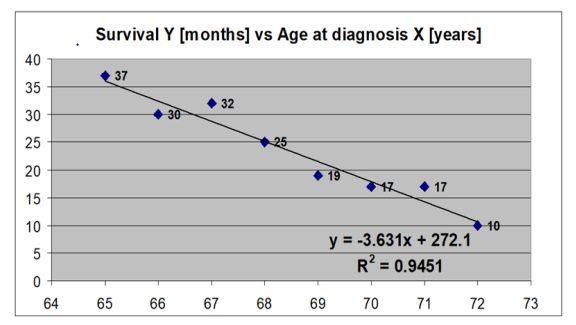
What is the main finding from simple linear regression model that is presented below? What does the coefficient of determination mean in this case? What is the value of the correlation coefficient in this case?

What is the main finding from simple linear regression model that is presented below? What does the coefficient of determination mean in this case? What is the value of the correlation coefficient in this case?

• Main finding: every 1 year increase in the age at diagnosis X is associated with a 3.63 decrease in the expected survival Y

• Coefficient of determination: it equals to -0.97

• Value: 94.5% of the variance in survival is explained by the age at diagnosis

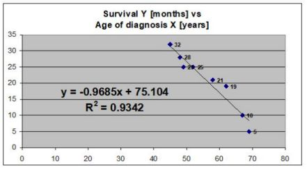
What is the is main finding from simple linear regression model that is presented below? What is the value of the correlation coefficient in this case?

What is the is main finding from simple linear regression model that is presented below? What is the value of the correlation coefficient in this case?

• There is a negative linear correlation between the age of diagnosis X (years) and Survival Y (months).

• The correlation of determination is 93.42%, this suggests that 93.42% of the variation of survival Y in months can be predicated from age of diagnosis in X in years. 6.58% variation of survival Y in months can not be predicted from age of diagnosis in X years.

• At the age of 0 the survival Y months would = 75.105. The value of correlation coefficient is r= - 0.967, this suggests a negative correlation.

• For every 1 year increase in age, there is a 0.9685 decrease in survival time.

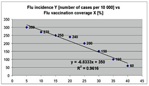
What is the is main finding from simple linear regression model that is presented below? What is the value of the correlation coefficient in this case?

What is the is main finding from simple linear regression model that is presented below? What is the value of the correlation coefficient in this case?

• There is a negative linear correlation between Flu incidence Y (number of cases per 10000) and Flu vaccination coverage X (%).

• The correlation of determination is 96.16%, this suggests that 96.16% of the variation Flu incidence Y (number of cases per 10000) can be predicated by Flu vaccination coverage X (%).

• 3.84% of the variation Flu incidence Y (number of cases per 10000) cannot be predicated by Flu vaccination coverage X (%) gym training per week X in hours.

• At the 0-flu vaccination coverage X the flu incidence Y
  (number of cases per 10000) will be 350.

• The value of correlation coefficient is r= - 0. 981, this suggests a
  negative correlation.

• For every 1 vaccination coverage the number of cases per 10000 would be decrease of
  6.8333 flu incidence.

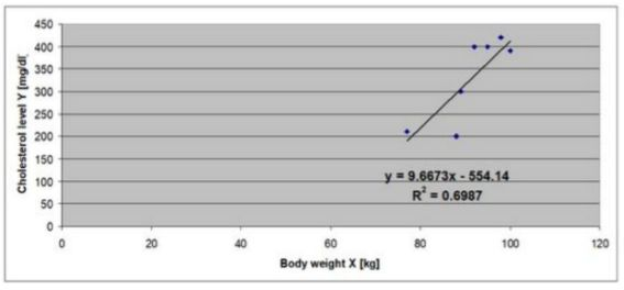
What is the is main finding from simple linear regression model that is presented below? What is the value of the correlation coefficient in this case?

What is the is main finding from simple linear regression model that is presented below? What is the value of the correlation coefficient in this case?

• Cholesterol level (mg/dl)

• Body weight x (kg)

What is the is main finding from simple linear regression model that is presented below? What is the value of the correlation coefficient in this case?

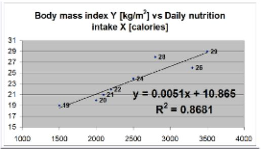
What is the is main finding from simple linear regression model that is presented below? What is the value of the correlation coefficient in this case?

• The graph shows the relationship between daily nutritional intake (X, in calories) and body mass index (Y, in kg/m²).

• For every 1 calorie increase in daily intake, the BMI increases by 0.0051 kg/m².

• The intercept (10.865) is the estimated BMI when daily caloric intake is zero (not realistic, but a part of the model).

• The coefficient of determination (R² = 0.8681) indicates that approximately 86.81% of the variation in BMI can be explained by daily nutritional intake. This is a strong relationship.

• To find the correlation coefficient r, take the square root of R² = 0.9318

• Since the slope is positive, the correlation is positive → strong positive correlation.

• Main finding: Higher daily caloric intake is strongly and positively associated with higher BMI.

What is the main finding from simple linear regression model that is presented below? What does the coefficient of determination mean? What is the value of the correlation coefficient in this case?

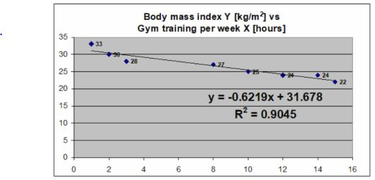
What is the main finding from simple linear regression model that is presented below? What does the coefficient of determination mean? What is the value of the correlation coefficient in this case?

• There is a negative linear correlation between body mass index Y (kg/m 2) and gym training per week X in hours.

• The correlation of determination is 90.45%, this suggests that 90.45% of the variation of body mass index Y (kg/m2) can be predicated by gym training per week X in hours.

• 9.55% variation body mass index Y (kg/m2) cannot be predicted by gym training per week X in hours.

• At the 0-gym training per week, the body mass index would be 31.678 kg/m2.

• The value of correlation coefficient is r= - 0.95, this suggests a negative correlation.

• For every 1 hour of gym training per week increase in age, there is a 0.6219 decrease in body mass index Y.

What is the value of the interquartile range for the variable presented on the boxplot below? What is the value of the most extreme outliers in this case? What is the distribution of this variable?

What is the value of the interquartile range for the variable presented on the boxplot below? What is the value of the most extreme outliers in this case? What is the distribution of this variable?

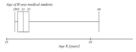
• IQR = 4 (23-19)

• Most extreme outlier: no lower outliers.

• There are upper outliers (>29 years)

• The destribution: right skewed destribution

• The interquartile range equals 4 years.

• There are no lower outliers.

• There are upper outliers (> 29 years).

• Upper outlier: Q3 + (1.5 x IQR) = 23 + (1.5 x 4) = 23 + 6 = 29. values between 29 and 48 are upper outliers.

• The distribution of this variable is right-skewed.

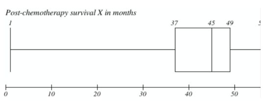
What is the value of the interquartile range of the post-chemotherapy survival in I stage breast cancer patients (presented on the boxplot below)? What is the value of the range of this variable? What is the
distribution of this variable?

What is the value of the interquartile range of the post-chemotherapy survival in I stage breast cancer patients (presented on the boxplot below)? What is the value of the range of this variable? What is the
distribution of this variable?

• IQR = 12 (49-37)

• The destribution: left skewed destribution

• The value of the range: 55

• IQR = 12

• Distribution of variable is left skewed.

• Range = 55

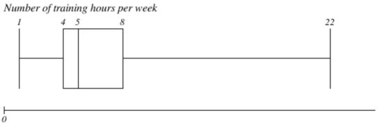
What is the value of the interquartile range of the weekly number of training hours in young adults (presented on the boxplot below)? What is the value of the most extreme outliers in this case? What is the distribution of this variable?

What is the value of the interquartile range of the weekly number of training hours in young adults (presented on the boxplot below)? What is the value of the most extreme outliers in this case? What is the distribution of this variable?

• IQR = 4 (8-4)

• The destribution: right skewed destribution

• Most extreme outlier: lower outlier (<7) and upper outlier (>18)

• IQR = 4

• Distribution of variable is right skewed.

• Range = 21 (22-1)

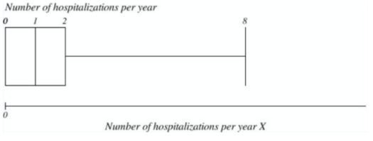
What is the value of the interquartile range for the number of hospitalizations per year in young adults (presented on the boxplot below)? What is the value of the most extreme outliers in this case? What is the distribution of this variable?

What is the value of the interquartile range for the number of hospitalizations per year in young adults (presented on the boxplot below)? What is the value of the most extreme outliers in this case? What is the distribution of this variable?

• IQR = 2 (2-0)

• The destribution: right skewed destribution

• Most extreme outlier: no lower outlier.

• There are upper outliers (>8)

• IQR= 2

• Distribution of variable right skewed.

• Extreme outlier: Lower outliers = -3, therefore there are no lower outliers.

• Upper outliers = 5, values between 5 and 8 are upper outliers.

• Lower outlier: Q1-(1.5 x IQR) = 0 - (1.5 x 2) = 0 - (3) = -3 - none

• Upper outlier: Q3 + (1.5 x IQR) = 2 + (1.5 x 2) = 2 + 3 = 5.

• values between 5 and 8 are upper outliers.

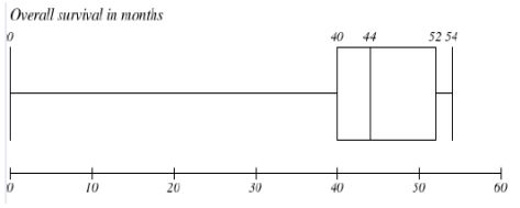
What is the value of the interquartile range for the overall survival in months (presented on the boxplot below)? What is the distribution of this variable? Are there any outliers in this data set and if yes, what are their values?

What is the value of the interquartile range for the overall survival in months (presented on the boxplot below)? What is the distribution of this variable? Are there any outliers in this data set and if yes, what are their values?

• IQR = 12

• Distribution of variable is left skewed.

• Lower outlier: Q1-(1.5 x IQR) = 0 - (1.5 x 12) = 0 - (18) = -18 - none

• Upper outlier: Q3 + (1.5 x IQR) = 52 + (1.5 x 12) = 52 + 18 = 70. none

When using x2-test, when and how do you apply the Yates correction?

When using x2-test, when and how do you apply the Yates correction?

• It is used only in a 2x2 contingency table (i.e., when both variables have 2 categories).

• Specifically applied in the Chi-square test for independence or goodness-of-fit when:

  • Sample size is small, especially when any expected frequency is less than 10 (some say < 5).

  • It helps to correct for overestimation of statistical significance in small samples.

• Yates correction adjusts for this by making the test more conservative, reducing the risk of a Type I error (false positive).

• Yates correction is applied to chi-square test in case of 1 degree of freedom

• Usual formula: χ2 = ∑ (O - E)²/E

• With Yate’s correcion: χ2 = ∑ (∣O − E∣ − 0.5)²/E

• O = observed frequency

• E = expected frequency

• 0.5 is the continuity correction (Yates’ adjustment)

• When there is only 1 degree of freedom, regular chi-test should not be used.

• Apply the yates correction by subtracting 0.6 from the absolute value of each calculated O-E term, then continue as usual with the new corrected values.

What is the main difference between parametric and non-parametric test? By what means you could check for it?

What is the main difference between parametric and non-parametric test? By what means you could check for it?

• Parametric Test assumes underlying distribution (usually normal)

• Non-Parametric Test - no assumption about data distribution

• Parametric Test requires interval or ratio (quantitative) data

• Non-Parametric Test can be used ordinal or nominal data

• Parametric Test based on means and standard deviations

• Non-Parametric Test based on medians and ranks

• Parametric Test e.g. t-test, ANOVA, Pearson correlation

• Non-Parametric Test e.g. Mann–Whitney U, Kruskal–Wallis, Spearman rank

• Main difference is that in the parametric test the sample is normally distributed in the population to which we plan to generalize the findings.

• In the non-parametric test, it is distribution free, no assumption about the distribution of the variable in the population.

• You need to check if data meet the assumptions of parametric tests, mainly normality and homogeneity of variance.

• Graphical methods:

  • Histogram (bell-shaped?)

  • Q–Q plot (data points lie on the line?)

• Statistical tests:

  • Shapiro–Wilk test (best for small samples)

  • Kolmogorov–Smirnov test

• If p-value < 0.05 → data not normal → use non-parametric test

• If p-value > 0.05 → data normal → can use parametric test

• Check for Homogeneity of Variance (if comparing groups):

  • Levene’s test or Bartlett’s test

  • If p < 0.05 → variances are unequal → parametric test may not be appropriate

A study on the level of obesity (defined as "underweight", "normal weight", "pre-obesity" and "obesity") in smokers and non-smokers came to the result of χ2 = 7.80 / df = 3. What is the p-value in this case and what does it mean? What conclusion can be drawn from this result?

A study on the level of obesity (defined as "underweight", "normal weight", "pre-obesity" and "obesity") in smokers and non-smokers came to the result of χ2 = 7.80 / df = 3. What is the p-value in this case and what does it mean? What conclusion can be drawn from this result?

• χ2 = 7.80

• Degrees of freedom = df = 3

• p > 0.05 tells us that if smoking status and weight category were truly independent in the population, we would see a chi-square statistic as large as 7.80 (or larger) about 5 % of the time purely by random sampling variation.

• We accept the null hypothesis.

• There is no association between smoking and level of obesity.

• The study does not provide statistically significant evidence that the distribution of weight categories differs between smokers and non-smokers.

The correlation between two variables is given by r = 0.0. What is the value of the coefficient of determination and why? Based on this what will be the best straight line through the data and why?

The correlation between two variables is given by r = 0.0. What is the value of the coefficient of determination and why? Based on this what will be the best straight line through the data and why?

• When r= 0.0 there is no linear association.

• The value of the coefficient of determination is (R²) = r² = 0.

• 0% of the variation in one variable can be explained by the other.

• There is no linear relationship between the two variables.

• R² is a proportion of variance in the dependant variable that is predictable from the independent variable.

• Therefore, there is no proportion in the dependant variable that is
  predictable from the independent variable.

• The best straight line through data would be a horizontal line (zero slope).

• When r = 0, the best-fitting line is the horizontal line at the mean of the dependent variable (Y): Y = Yˉ

• Because no linear trend exists between X and Y, the line that minimizes the total squared error (least squares regression) is simply the average of all Y-values.

• This line reflects that X gives no information about Y.

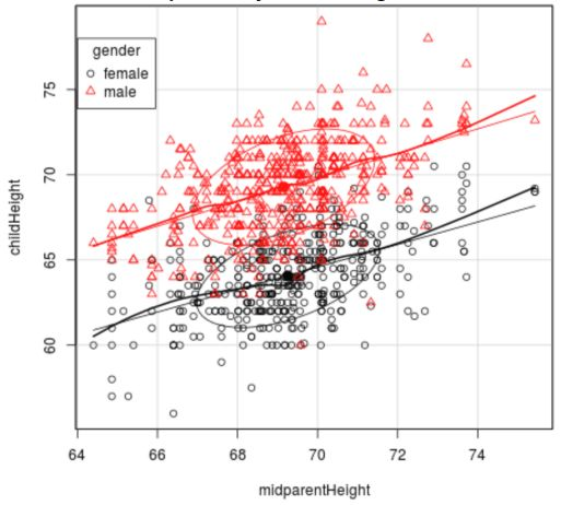
The scatterplot shows child's heights (y axis) versus parents’ heights (x axis) for a sample of 934 children in 205 families. Based on the scatterplot, what is the problem with using a regression equation for all 934 children? The correlation between father’s heights and male children’s heights is r=0.669. What is the proportion of variation explained by father’s heights?

The scatterplot shows child's heights (y axis) versus parents’ heights (x axis) for a sample of 934 children in 205 families. Based on the scatterplot, what is the problem with using a regression equation for all 934 children? The correlation between father’s heights and male children’s heights is r=0.669. What is the proportion of variation explained by father’s heights?

• Because of the large sample there are a lot of data points close together/ a lot of overlap.

• Making it difficult to analyse the individual results.

• When r= 0.669, there is a positive correlation.

• R2 = 0.448.

• Therefore, 44.8% of the variation in male children’s height can be predicted from the father’s height.

• This means that 55.2% of the variation in male children’s height can not be predicted from the father’s height.

What is the value of the interquartile range for the age of II year medical students (presented on the boxplot here)? What is the value of the range for this variable? What is the distribution of this variable?

What is the value of the interquartile range for the age of II year medical students (presented on the boxplot here)? What is the value of the range for this variable? What is the distribution of this variable?

• Every 1 year increase in the age at diagnosis, X will be associated with 3.631 months decrease in the expected survival rate Yt.

• 94.5% of the expected survival rate Yt could be predicted by the age at diagnosis X.

• IQR = Q3 − Q1

• Range = Max − Min

Which data grouping approach results in more precise estimates at the end? Why? Could you remove outliers from the data in order to get more precise estimates?

Which data grouping approach results in more precise estimates at the end? Why? Could you remove outliers from the data in order to get more precise estimates?

• Stratified sampling usually results in more precise estimates compared to simple random sampling or other grouping methods.

• In stratified sampling, the population is divided into homogeneous subgroups (strata) based on key characteristics (e.g., age, gender, income).

• Samples are then taken proportionally from each stratum.

• This reduces variability within each subgroup, leading to a lower overall variance in the estimate.

• As a result, estimates from stratified samples tend to be more precise (smaller standard error).

• Removing outliers can reduce variability in the data, which may improve precision (narrower confidence intervals, smaller standard errors).

• Outliers can distort the mean and variance, so cleaning data can help better represent the “typical” values.

• Outliers might represent real and important variations in the population.

• Removing them without justification can lead to biased estimates and loss of important information.

• The decision to remove outliers must be based on clear criteria (e.g., measurement error, data entry mistakes) and should be reported.

When describing a sample, what are the main advantages and disadvantages of the mean and median?

When describing a sample, what are the main advantages and disadvantages of the mean and median?

• MEAN Advantages

  • Uses all data points, so reflects total magnitude

  • Useful for further calculations (e.g., variance, standard deviation)

• MEAN Disadvantages

  • Sensitive to outliers and skewed data, which can distort the mean

  • Not always representative if data is skewed

• MEDIAN Advantages

  • Not affected by extreme values (outliers)

  • Represents the typical value in skewed data

• MEDIAN Disadvantages

  • Does not use all data points

  • Less useful for further mathematical operations

When applying the χ2-test, how could you correct the results if more than 1/5 of the expected categories are less than 5?

When applying the χ2-test, how could you correct the results if more than 1/5 of the expected categories are less than 5?

• Combine Categories

  • Merge some adjacent or similar categories to increase the expected frequencies.

  • This reduces the number of categories but ensures that each combined category has an expected count ≥ 5.

  • After merging, recalculate the expected frequencies and perform the χ² test again.

• Use Fisher’s Exact Test

  • For small samples or tables with low expected counts (especially in 2x2 tables), use Fisher’s Exact Test instead of χ².

  • Fisher’s test is exact and does not rely on large-sample approximations.

• Use Alternative Tests

  • Consider likelihood ratio chi-square test (G-test), which can sometimes be more reliable with small expected counts.

  • Or use Monte Carlo simulations to estimate p-values.

A study on the association between the degree of obesity and the incidence of pollen allergy in the general population came to a x2 = 9,488 (df = 4). What did the study conclude?

A study on the association between the degree of obesity and the incidence of pollen allergy in the general population came to a x2 = 9,488 (df = 4). What did the study conclude?

• Chi-square statistic: χ2 = 9.488

• Degrees of freedom (df) = 4

• The critical value for α = 0.05 and df = 4 is 9.488.

• Since the calculated χ2\chi^2χ2 value (9.488) is equal to the critical value at the 5% significance level,

• The p-value is approximately 0.05.

• p = 0.05, so we accept the null hypothesis

• There may be an association between obesity and pollen allergy, but evidence is weak.

A study on the association between the degree of obesity and the incidence of pollen allergy in the general population came to a x2 = 11.071 (df = 5). What did the study conclude?

A study on the association between the degree of obesity and the incidence of pollen allergy in the general population came to a x2 = 11.071 (df = 5). What did the study conclude?

• Chi-square statistic: χ2 = 11.071

• Degrees of freedom: df = 5

• The critical value for χ2 with df = 5 at α = 0.05 is 11.070.

• Since χ2=11.071 is just slightly above the critical value,

• The p-value is approximately 0.0499, which is just below 0.05.

• P value is less than 0.05 so therefore we reject the null hypothesis and accept the alternative hypothesis.

• there is a statistically significant association between the degree of obesity and the incidence of pollen allergy amonst the general population

Which are the types of scientific research?

Which are the types of scientific research?

• Quantitative = The expectation of success empirically is so unlikely that its exact probability cannot be calculated.

• Qualitative Definition = Any treatment that merely preserves permanent unconsciousness or total dependence on intensive medical care.

• PRIMARY AND SECONDARY

• APPLIED AND BASIC

• DESCRIPTIVE AND CASUAL

• DEDUCTIVE AND INDUCTIVE

Explain the methodology of scientific research:

Explain the methodology of scientific research:

• Steps of scientific research include making observations and asking questions, forming a hypothesis based on these questions, making predictions and testing.

• These predictions and using the result to make new hypotheses or predictions.

How can we reduce the width of the confidence interval? What are the advantages and disadvantages?

How can we reduce the width of the confidence interval? What are the advantages and disadvantages?

• Larger samples reduce the standard error, narrowing the CI.

  ✅ Advantage: Improves precision without reducing confidence.

  ❌ Disadvantage: May be costly, time-consuming, or impractical.

• A lower confidence level reduces the Z-score or t-score

  ✅ Advantage: Narrows the CI and gives a more precise interval.

  ❌ Disadvantage: Increases the risk of Type I error (less confidence that the interval contains the true population parameter).

A study on the level of physical activity (measured as a weekly number of training hours) of undergraduate and postgraduate students came to the result of t = 1.96. What did the study conclude?

A study on the level of physical activity (measured as a weekly number of training hours) of undergraduate and postgraduate students came to the result of t = 1.96. What did the study conclude?

• For a two-tailed test at the 5% significance level (α = 0.05): The critical t-value is approximately ±1.96 (for large sample sizes; exact value depends on degrees of freedom).

• Since the calculated t = 1.96 is equal to the critical value, the p-value is approximately 0.05.

• This is right at the threshold for statistical significance.

• The study concludes that there is a 95% level of confidence meaning that the two samples are statistically significant.

• We assume the sample size is large if it has 95% confidence level at t=1.96 the p-value is less than 0.05 so we reject the null hypothesis so there is a significant difference

• When t= 1.96, p= 0.05, therefore accept H0 and reject H1

• There is no significant association between the undergraduate and postgraduate students

Suppose that a medical study found a statistically significant relationship between wearing gold jewelry and developing skin cancer. Suppose the study was based on a sample of 100,000 people and had a p-value of 0.049. How would you react to these results?

Suppose that a medical study found a statistically significant relationship between wearing gold jewelry and developing skin cancer. Suppose the study was based on a sample of 100,000 people and had a p-value of 0.049. How would you react to these results?

• 1p-value usually holds a statistically significance, and the sample size is sufficient enough for reliability.

• So there is a low probably for the hypothesis to be rejected.

• If p< 0.05, we reject H0 and we accept H1.

• Therefore, there is significant association between wearing gold jewellery and developing skin cancer.

• The p-value = 0.049 means that, assuming no real relationship exists between wearing gold jewelry and developing skin cancer, there's a 4.9% chance of observing a result this extreme just by random chance.

• Since p < 0.05, the result is considered statistically significant at the 5% level.

• Very large sample size (n = 100,000)

  • With such a big sample, even tiny and possibly meaningless differences can become statistically significant.

  • The study may detect a statistically significant effect that is not practically important.

Deletion of outlier data is generally a controversial practice. However, you have the full right to remove outliers in one specific case. What is this case?

Deletion of outlier data is generally a controversial practice. However, you have the full right to remove outliers in one specific case. What is this case?

• Deletion of outlier data is a controversial practice but can occur for several reasons: invalid data entry, random chance, skewed distribution, experimental error. You can eliminate outliers only when you do not get the result you want.

• In case of obvious mistakes in the data collection process. For example, wrong value measurement, invalid data entry, etc.

When grouping quantitative data, what are the main advantages and disadvantages of the classes of values and classes of intervals?

When grouping quantitative data, what are the main advantages and disadvantages of the classes of values and classes of intervals?

• Classes of Values Advantages

  • Exact values preserved: No loss of detail or precision.

  • Easy to interpret when there are few distinct values.

  • Useful for discrete data.

• Classes of Values Disadvantages

  • Can create too many groups if data have many unique values, making analysis and visualization harder.

  • Not practical for large datasets with continuous variables.

• Classes of Intervals Advantages

  • Simplifies data by reducing the number of groups.

  • Easier to visualize and interpret overall trends.

  • Useful for continuous data or large datasets.

  • Helps in detecting distribution patterns.

• Classes of Intervals Disadvantages

  • Loss of detail and precision because individual values are grouped.

  • Choice of interval width and boundaries can be arbitrary and affect results.

  • May hide important data features or outliers within intervals.

Which data grouping approach results in more precise estimates at the end? Why? Could you remove outliers from the data in order to get more precise estimates?

Which data grouping approach results in more precise estimates at the end? Why? Could you remove outliers from the data in order to get more precise estimates?

• Stratified grouping (stratified sampling) generally results in more precise estimates than simple grouping or random sampling.

• Stratified grouping divides the population into homogeneous subgroups (strata) based on characteristics relevant to the study (e.g., age, gender).

• Within each stratum, data tend to be more similar, reducing variability within groups.

• This lowers the overall variance and increases precision of estimates when the strata are combined properly.

• Compared to grouping by arbitrary intervals or values, stratification targets known sources of variation, improving accuracy.

• Outliers caused by measurement errors or data entry mistakes can distort results and increase variability.

• Removing these justified outliers reduces variance, leading to more precise estimates.

• If outliers represent true, natural variability in the population, removing them can bias results.

• Arbitrary removal of outliers can lead to misleading conclusions.

A study on the level of physical a activity (measured as a weekly number of training hours) of undergraduate and postgraduate students came to the result of t = 2.96. What is the p-value in this case and what does it mean? What conclusion can be drawn from this result?

A study on the level of physical a activity (measured as a weekly number of training hours) of undergraduate and postgraduate students came to the result of t = 2.96. What is the p-value in this case and what does it mean? What conclusion can be drawn from this result?

• If t= 2.96, p> 0.05. This means that we accept the H0, and we reject the H1

• There is no association of the level of physical activity between undergraduate and postgraduate students.

A study on the level of physical activity (measured as a weekly number of training hours) of undergraduate and postgraduate students came to the result of t = 1.96. What did the study conclude?

A study on the level of physical activity (measured as a weekly number of training hours) of undergraduate and postgraduate students came to the result of t = 1.96. What did the study conclude?

• If t= 1.96, p= 0.05. This means that we accept the H0.

• There is no significant association between the physical activity of undergraduate and postgraduate students.

A study on the level of physical activity (measured as a weekly number of training hours) of undergraduate and postgraduate students came to the result of t = 2.96. What did the study conclude?

A study on the level of physical activity (measured as a weekly number of training hours) of undergraduate and postgraduate students came to the result of t = 2.96. What did the study conclude?

• If t= 2.96, p> 0.05. This means that we accept the H0, and we reject the H1.

• There is no association of the level of physical activity between undergraduate and postgraduate students.

What are the main differences between the standard deviation (SD) and the standard error of the mean (SEM)? Outline and explain these differences.

What are the main differences between the standard deviation (SD) and the standard error of the mean (SEM)? Outline and explain these differences.

• The standard deviation (SD) measures the amount of variability, or dispersion, from the individual data values to the mean, while the standard error of the mean (SEM) measures how far the sample mean of the data is likely to be from the true population mean.

• The (SEM) = always smaller than (SD).

• SD tells you about the variability in your sample or population data.

• SEM tells you how precisely your sample mean estimates the population mean.

What are the main differences between the x2-test and the Fischer's exact test? Outline and explain these differences.

What are the main differences between the x2-test and the Fischer's exact test? Outline and explain these differences.

• Use χ² test for larger samples with expected counts ≥ 5.

• Use Fisher’s Exact test for small samples or when expected counts are too low for χ² to be reliable.

• Sample size:

  • χ²: Requires large samples, expected counts ≥ 5

  • Fisher: Suitable for small samples, low expected counts

• Data type:

  • Both used for categorical data, mainly 2x2 tables

• Calculation:

  • χ²: Approximate test using chi-square distribution

  • Fisher: Calculates exact probability

• When to use:

  • χ²: Large samples with sufficient expected frequencies

  • Fisher: Small samples or when χ² assumptions violated

• Computation:

  • χ²: Fast and simple

  • Fisher: Computationally intensive for large tables

• Accuracy:

  • χ²: Less accurate with small or sparse data

  • Fisher: More accurate for small data sets

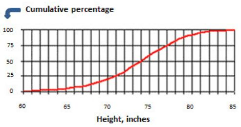
Below, the cumulative frequency (in red) plot shows height (in inches) of college basketball players. What is the interquartile range of the height? (6 Points)

Below, the cumulative frequency (in red) plot shows height (in inches) of college basketball players. What is the interquartile range of the height? (6 Points)

• IQR = Q3 - Q1 = (value of 75% percentile) - (value of 25% percentile)

• IQR = Q3 - Q1 = 77 - 71 = 6

When standardizing indicators of two samples, could you switch standards? What will happen if standards are switched? (6 Points)

When standardizing indicators of two samples, could you switch standards? What will happen if standards are switched? (6 Points)

• You can switch standards in standardization.

• Z-scores depend on the chosen standard (mean & SD).

• Switching standards changes the reference distribution.

• This affects the scale and meaning of standardized scores.

• Comparisons between samples become asymmetric depending on standard used.

• Interpret results carefully, specifying which standard was applied.

How decreasing the Z-score will affect the precision of the population estimate? (6 Points)

How decreasing the Z-score will affect the precision of the population estimate? (6 Points)

• A smaller Z-score results in a narrower confidence interval around the estimate.

• Because the interval is narrower, the estimate appears more precise.

• However, this increased precision comes at the cost of being less confident that the interval contains the true population parameter.

• There's a trade-off between precision and confidence — decreasing the Z-score increases precision but reduces certainty.

• Since the Z-score is part of the margin of error formula (Z × standard error), lowering Z decreases the margin of error.

• While precision increases, the reliability of the estimate (i.e., how often it would capture the true value in repeated samples) decreases.

A study on the rate of physical activity of smokers and non-smokers came to t = 1.62. What did the study conclude? (6 Points)

A study on the rate of physical activity of smokers and non-smokers came to t = 1.62. What did the study conclude? (6 Points)

• When t = 1.62, p > 0.05

• We accept the null hypothesis, therefore there is no significant association between the rate of physical activity of smokers and of non-smokers.

A study on the level of obesity (defined as “underweight”, “normal weight”, “pre-obesity” and “obesity”) in smokers and non smokers came to the result χ2 = 7.80 / df = 3. What is the p-value in this case and what does it mean? What conclusion can be drawn from this result? (6 Points)

A study on the level of obesity (defined as “underweight”, “normal weight”, “pre-obesity” and “obesity”) in smokers and non smokers came to the result χ2 = 7.80 / df = 3. What is the p-value in this case and what does it mean? What conclusion can be drawn from this result? (6 Points)

• χ2 = 7.80 / df = 3 => p > 0.05

• We accept the null hypothesis.

• There is no association between smoking and level of obesity.

Does the sample size affect the probability of type II error? Does the sample size affect the probability of type I error? Explain your response. (6 Points)

Does the sample size affect the probability of type II error? Does the sample size affect the probability of type I error? Explain your response. (6 Points)

• A type II error is when a false null hypothesis is incorrectly retained.

• Power is inversely proportional to the probablity of making a type II error, and power itself is dependent on sample size, so yes, sample size does affect the probablity of making a type II error

• Larger sample size = high power = lower probability of type II error.

• A type I error is the incorrect rejection of a true null hypothesis

Mean weight of 500 male volleyball players is found to be 93 kg with a standard deviation of 6 kg. Data are normally distributed. The number of volleyball players from this sample whose weight is more than 99 kg is equal to:

Mean weight of 500 male volleyball players is found to be 93 kg with a standard deviation of 6 kg. Data are normally distributed. The number of volleyball players from this sample whose weight is more than 99 kg is equal to 80

• Mean (μ) = 93 kg

• Standard deviation (σ) = 6 kg

• Sample size (n) = 500

• We want to find how many players weigh more than 99 kg.

• Z = (99 - 93)/6 = 1

• P (Z > 1) = 1 - P(Z ≤ 1) = 1 - 0.8413 = 0.1587

• Number of players = 0.1587 × 500 = 79.35 ≈ 79

• 79 volleyball players are expected to weigh more than 99 kg.

If all the values of a data set are the same, the standard deviation is equal to:

If all the values of a data set are the same, the standard deviation is equal to zero

Mean birth height of 600 newborns is found to be 50 cm with a standard deviation of 2 cm. Data are normally distributed. The number of newborns from this sample whose birth height is more than 54 cm or less than 46 cm is equal to:

Mean birth height of 600 newborns is found to be 50 cm with a standard deviation of 2 cm. Data are normally distributed. The number of newborns from this sample whose birth height is more than 54 cm or less than 46 cm is equal to 30

• Mean (μ) = 50 cm

• Standard deviation (σ) = 2 cm

• Sample size (n) = 600

• We are asked to find how many newborns have a birth height > 54 cm or < 46 cm

• For 54cm: Z = (54 - 50)/2 = 2

• For 46cm: Z = (46 - 50)/2 = -2

• P (Z > 2) = 0.0228

• P (Z < -2) = 0.0228

• P(Z > 2 or Z < −2) = 0.0228 + 0.0228 = 0.0456

• 0.0456 × 600 = 27.36 ≈ 27

• 27 newborns are expected to have a birth height greater than 54 cm or less than 46 cm.

If all the values of X are increased 10 times, then the standard deviation:

If all the values of X are increased 10 times, then the standard deviation:

As standard deviation is invariant to the change of origin, standard deviation will remain same