Elementary Statistics for Psychology

Flash Cards for PBSI 301

Statistics

Statistics is a set of tools and techniques used for describing, organizing, and interpreting information or data.

Why do we need Statistics? (Ch. 1)

To describe, predict, and explain behaviours or trends.

Descriptive Statistics (Ch. 1)

Used to organize and describe data.

Examples: What is the most common major? What is the average age? What is the most popular baseball team? (They use counts, means, percentages, etc…)

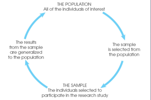
Inferential Statistics (Ch. 1)

Inferential statistics allow you to INFER the truth about the larger group (population) based on the information you gather from this smaller group of people (sample).

(Done after description.)

Population (Ch. 1)

The group you are actually interested in drawing some conclusions about.

Sample (Ch. 1)

It is a subset containing the characteristics of our population, the individuals selected to make conclusions for our population.

Variable (Ch. 1)

Something that can change (vary) or have different values for different individuals. Variables represent the concepts we are interested in. (i.e age, height, major, etc…).

Data (Ch. 1)

Information collected from the sample on the variables we are interested in. The actual numbers, measurements, or characteristics that represent the ideas we are interested in.

Continuous Data (Quantitative) (Ch. 1)

Data measured in a continuum like height, weight, age, etc. All numbers between two endpoints are possible scores.

Categorical data (Ch. 1)

Data that sorts people into categories, like major, eye color, ethnicity, etc.

Measures of Central Tendency (Ch. 2)

Mean, median, mode.

The mean (Ch. 2)

The most familiar measure of central tendency also known as the “average”. The mean is sensitive to extreme scores.

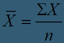
Formula for the mean (Ch. 2)

“X bar” is the symbol for the mean

X is each individual score in the group (the data)

“Σ” or “Sigma” is the summation sign

• When you see a sigma, you should sum whatever follows it n is the sample size. So when you see ΣX, you sum up all individual scores in the data.

The median (Ch. 2)

The median is the midpoint in a set of scores. The median is not affected by extreme scores.

To find the median (Ch. 2)

To find the median you have to list the values in order (either highest to lowest or lowest to highest) then find the middle-most score. If there is no middle score, add the two nearest middle scores and divide by 2.

Percentile points (Interquartile range or IQR) (Ch.2)

Refers to the percentage of cases equal to and below a certain point in a group of scores. The median is always the 50% percentile.

The mode (Ch. 2)

The mode is the value that occurs most frequently in the data set. Not affected by extreme scores, just count how many times each value appears. Used in categorical dats usually.

Bimodal (Ch. 2)

There can be more than 1 mode—this is referred to as a bimodal data set.

When do we use each measure of central tendency (Ch. 2)

1. Use the mode when the data are categorical

2. Use the mean when the data are continuous and you have no (or very few) extreme scores

• By far the most common measure of central tendency in psychology

3. Use the median when the data are continuous and you think the mean is misleading because of extreme scores

• When in doubt—report both!

Weighted mean (Ch. 2)

Shortcut for calculating the mean in a large data set in which certain values show up multiple times

• List all the values in the sample

• List how often each value occurs

• Multiply the values by their frequency

• Sum all the values in the value times the frequency column

• Divide by total frequency

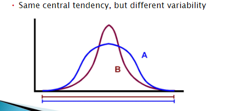
Variability (Ch.3)

Tell us how different the scores are from each other. Represent the spread or dispersion in the dataset. Variability helps us understand the nature of our sample and the nature of our variables.

Why is variability important? (Ch. 3)

Different variables within the same sample may have different variability and tells us how much spread or dispersion (variability) there is in a data set.

Measures of variability (Ch.3)

Range, standard deviation (SD), and variance.

Range (Ch.3)

The most general measure of variability. Gives an idea of how far apart the scores are from each other. Computed by subtracting the lowest score from the highest score.

• r = h – l

• r = range

• h = highest score in the data set

• l = lowest score in the data set

(Always give the minimum and maximum values when reporting the range. This provides some context for the range.)

Problems with range (Ch.3)

• These 2 samples would have the same range

• Ignores the middlemost values

• Considers only the most extreme scores

Standard deviation (Ch. 3)

The most common measure of variability. Represents the average amount of variability in a set of scores. Its sensitive to extreme scores.

• A small/low standard deviation value indicates that most data points tend to be close to the mean

• A large/high standard deviation value indicates that most data points tend to be far away from the mean

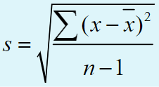
Calculating standard deviation (Ch. 3)

• s = Standard deviation (also SD)

• √ = square root (find the square root of what follows)

• ∑= summation (find the sum of what follows)

• x = each individual score

• X bar = mean of all the scores on x

• n = sample size

1. List all the scores 2. Compute the mean 3. subtract the mean from each score (x-xbar) 4. Square all the differences 5. Sum all the squared deviations 6. Divide the sum of squares by n-1. 7. Compute the square root of what is left.

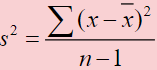
Variance (Ch. 3)

The third measure of variability. If you know the standard deviation, then you know the variance. Variance rarely reported as a descriptive statistic.

Outlier (Ch. 3)

A data point that appears to deviate markedly from the other data points in the sample. anything more than 2 standard deviations away from the mean is a potential outlier. A data point more than 3 standard deviations from the mean is a likely outlier.

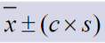
To find outliers (Ch. 3)

• X-bar = mean

• c = cut off value of interest

• s = standard deviation

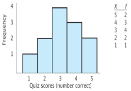
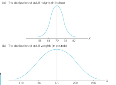
Histograms (Ch. 4)

Histograms allow us to see the distribution of our data. In a histogram, the height of each bar is the number of times each value occurs in our data set.

Distributions can vary in 4 ways;

• Central tendency

• Variability

• Skewness

• Kurtosis

(Bar graphs ≠ histograms. Bar graphs show the frequency of categorical responses. Histograms show the distribution of continuous variables).

• Note that the y and x-axis can be altered to show a misleading graph.

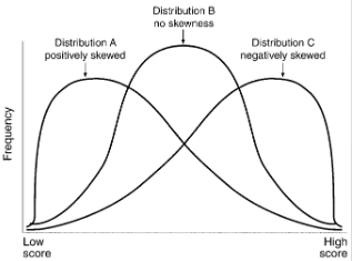
Symmetrical vs. Skewed Distributions (Ch. 4)

• Symmetrical Distributions: If you fold the graph in half, the two halves look the same. Mean, median, and mode are in the middle.

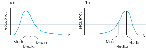
• Skewness: Refers to lack of symmetry. Asymmetrical or lopsided. “Piling up” of X values on one side of the distribution. Positive and negative skewness (AKA Right skewed or left skewed). Mean, median, and mode differ.

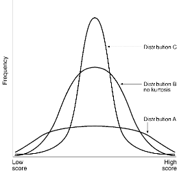
Kurtosis (Ch. 4)

Refers to how peaked vs. flat the distribution.

• Platykurtic = LOW kurtosis. Relatively flat (more variability).

• Leptokurtic =HIGH kurtosis. Relatively peaked (less variability).

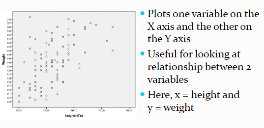
Correlations (Ch. 5)

AKA what is the relationship between these two variables. We can compute a correlation when we have scores on two variables (x and y) from each member of our sample.

Correlation coefficients (Ch. 5)

Correlation coefficients assign a single number to describe the relationship between two variables. Abbreviated as r and ranges from -1 to 1. The coefficient tells us direction (positive or negative)and strength ( Strong, moderately strong, and weak.)

Direction (Ch. 5)

Positive or Negative

• + signs indicate positive (or direct) relationships. Scores on the variables move in the same direction.

• - signs indicate negative (or indirect) relationships  Scores on the variables move in opposite directions.

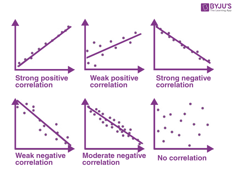
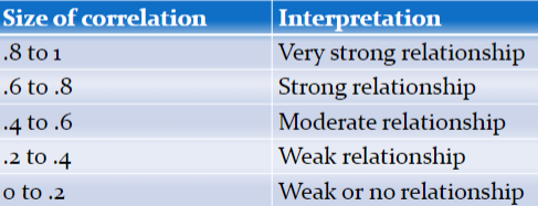
Strength (Ch. 5)

The magnitude of the coefficient (or how far it is from zero) tells us how strong the relationship is.

• If r = 0, then no relationship

• If r = -1 or 1, then perfect relationship

• The closer r gets to an absolute value of 1, the closer it is to a perfect relationship

( Perfect Relationship (r=+/-1) and no correlation r= 0)

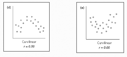
Limitations of correlation coefficients (Ch. 5)

• The correlation coefficient can only be used to identify linear relationships.

• Can be curvilinear

• There could be restrictions on the range

  • Occurs when most subjects have similar scores on one of the

  variables being correlated

  • The value of the correlation coefficient is reduced and does

  not capture the true relationship between the variables

• Lastly, outliers.

Curvilinear (Ch. 5)

The variables below definitely have a relationship, but the correlation coefficient will not find it.

• Note that r = 0 for both of these pictures.

Coefficient of determination (Ch. 5)

The coefficient of determination represents how much variation 2 variables share (in percentages)

• In other words, how much of the variance in variable X can be accounted for, or is shared, by the variance in Y (and vice-versa)

• Another way to say how much 2 variables have in common

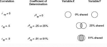
Coefficient of determination pt. 2 (Ch. 5)

The more 2 variables have in common, the more variance they will share.

• But even strong relationships (like the one we calculated, r = .61) have a lot of variance leftover (100% – 37%)

• 63% of the variance in Y is accounted for by factors OTHER than X.

• This variance that is leftover is called the coefficient of alienation.

Correlation v. causality (Ch. 5)

Correlation DOES NOT EQUAL causation. We can never definitively assume causation from a correlational relationship.

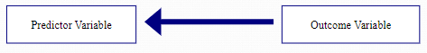
Reverse causation (Ch. 5)

The causal direction may be opposite from what has been hypothesized.

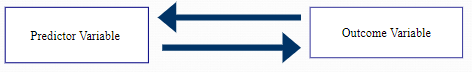
Reciprocal causation (Ch. 5)

Two variables cause each other. (“Spiral effect”/cyclical)

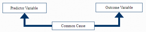
Common casual variables (Third variables) (Ch. 5)

Some unknown third variable is actually influencing the two variables in the correlation.

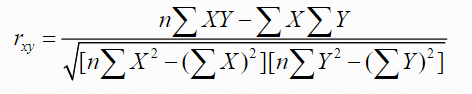
Computing a correlation coefficient (Ch. 5)

• rxy = the correlation between x and y

• n is the sample size

• X is each individual's score on the X variable

• Y is each individual’s score on the Y variable

• XY is the product of each X score times its corresponding Y score

• X2 is each individual's X score squared

• Y2 is each individual’s Y score squared

Measurement (Ch. 6)

The act or process of assigning numbers to phenomena according to a rule.

Properties of measurements / scales (Ch. 6)

The type of scale we use has important implications for what kind of statistics we use.

• Nominal scales

• Ordinal scales

• Interval scales

• Ratio scales

Nominal scales (Ch. 6)

Categorical. The categories must be mutually exclusive. Data is in the form of counts/percentages. Nominal = nameable

Ordinal scales (Ch. 6)

The number is a ranking. Not clear how much “distance” separates the data points on the scale. Ordinal = ordering.

Interval scales (Ch. 6)

Ordered events with equal spacing (based on an underlying continuum). Zero (0) not necessarily meaningful • May not even be part of the potential range. EQUAL INTERVALS.

Ratio scales (Ch. 6)

Similar to interval scale, but 0 has a specific meaning. zerO = ratiO

• 0 = the complete absence of the attribute

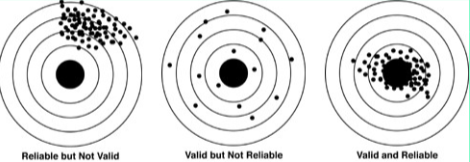
Reliability vs validity (Ch. 6)

• Reliability: How do I know that the measure I use works consistently?

• Validity: How do I know that the measure I use measures what it is supposed to (i.e., accuracy)?

Observed v. true scores (Ch. 6)

• Observed score = the score you actually got

• True score = the true reflection of what you really know

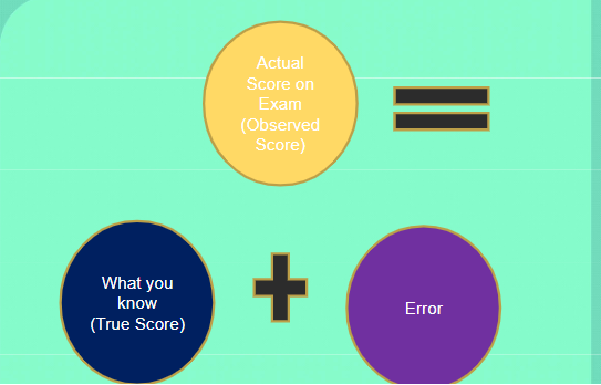
Error score (Or “measurement error”) (Ch. 6)

Discrepancy between observed score and true score. The less error the more reliable/valid the measure can be.

Reliability (Ch. 6)

The consistency or reproducibility of a measure or method.

4 types-

• Test-retest

• Parallel forms

• Internal consistency reliability - assessed by Cronbach’s Alpha (α)

• Inter-rater

Validity (Ch. 6)

How accurately a method measures what it is intended to measure.

3 types-

• Content

• Criterion

• Construct

Criterion validity (Ch. 6)

2 other sections/ divisions: Examples-

• Concurrent Validity: Does the measure correlate with

  grades in PSBI 301? Class attendance? Etc.

• Predictive Validity: Does the measure predict who will

  have a job using stats 10 years from now?

Construct validity (Ch. 6)

2 other sections/ divisions: Examples-

• Convergent Validity- Does the measure relate to other things it should?

• Discriminant Validity- Does the measure NOT relate to things it shouldn’t?