IIoT PDF 15: Machine Learning (Slides: 51-82)

Definition and short note descriptions

Artificial Neural Networks (Slide: 51)

Non-mandatory rule:
No. of hidden layers → b/w no. of inputs and outputs of the model

• Classical Neural Networks: 1-2 hidden layers

• Deep learning: Many hidden layers

• Type of ML model inspired by the structure and function of the human brain

• Used for complex tasks such as image recognition, speech recognition, and predictive maintenance in industrial automation

• Consists of 3 layers: (i) Input layer (ii) Hidden Layer (iii) Output Layer

• Can model complex, non-linear relationships in data.

• Require large amounts of labeled data for training.

• Used in industrial automation for tasks like quality inspection, anomaly detection, and predictive maintenance.

How it works:

• Each neuron receives inputs, multiplies them by weights, adds a bias, and passes the result through an activation function (such as ReLU or sigmoid).

• The network learns by adjusting the weights and biases during training to minimize the error between its predictions and the actual results (using algorithms like backpropagation and optimizers such as SGD or Adam).

Artificial Neural Networks: Layers (Slide: 51)

1. Input Layer

2. Hidden Layers

3. Output Layer

1. Input Layer
   Depends exclusively on the no. of features of the training data
   

2. Hidden Layers
   Required if the data is not linearly separable.
   No. of hidden layers depends on complexity of the data “
   

3. Output Layer
   No. of nodes depends on whether:

   • it is a “regression”/ a “binary classification” - output then contains only one node

   • “Multiclass classifier” - output then has as many nodes as the no. of classes or less

Equation for one neuron [Slide: 53,56]

If the input layer has values x1 and x2, weights w1 and w2, and bias b, then:

• Weighted Sum (z) = w1 x1 + w2 x2 + b

• Activation function (a) = ReLU(z) = max(0, z)

Typical activation function for hidden layers: ReLU - Rectified Linear Unit

f(x) = 0, for x < 0
f(x) = x for x>=0

Derivative
f(x) = 0 for x < 0
f(x) = 1 for x >= 0

Activation Functions in Neural Networks [Slide: 54]

• Mathematical gate attached to each neuron that decides whether it should "fire" or pass its signal forward.

• Introduces non linearity, allowing the network to learn complex, real world patterns.

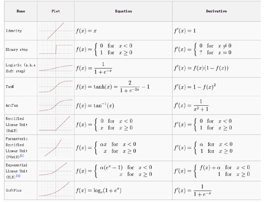
Activation Functions in output layer for classification

1. Binary classification: Sigmoid

2. Multiclass Classification: Softmax [Slide: 57

1. Binary classification: Sigmoid
   Converts a real valued number into a strict range between 0 and 1
   

2. Multiclass classification: Softmax
   Converts a vector of real numbers (often called "logits") into a probability distribution
   

How does a neural network learn? [Slide: 63]

• Use a lot of training data, i.e. images which are labeled (e.g. of handwritten digit recognition: Images containing handwritten digits and digital labels indicating which digits each image is supposed to represent)

• Start with randomly chosen values for all parameters

• The result is a vector containing incorrect probabilities for the different classes

MINI-BATCHES (SGD), ITERATIONS & EPOCHS

Why are mini batches needed? [Slide: 65]

• Huge training datasets are needed to calculate a huge amount of parameters

• Calculating with the entire huge training dataset would require a huge amount of computer memory and of computing power, the later resulting in extremely long update cycles.

• Calculating the training for only one image at a time would be too slow

MINI-BATCHES (SGD), ITERATIONS & EPOCHS

What are mini batches? [Slide: 65]

• Training dataset is randomly shuffled

• Training set is divided into mini batches, sometimes, e.g. in YOLO, called batches (e.g. entire training dataset = 1044 images → 8 mini batches = 128 images each;
  
  (Batch is size is often an exponential of 2 as that uses memory efficiently. The remaining images will likely be used in the next epoch cycle after the training datasets have been reshuffled).

MINI-BATCHES (SGD), ITERATIONS & EPOCHS

What are iterations? [Slide: 65]

• Training is done for one mini batch including calculation of forward pass, loss function, backpropagation and optimizer, updating the weights and bias values for this mini batch. This whole step is called 1 Iteration or a training step.

• These iterations are processed for all other mini batches (1 iteration for 1 mini batch; each time updating the weights)

MINI-BATCHES (SGD), ITERATIONS & EPOCHS

What is an epoch? [Slide: 65]

• The process from shuffling the training datasets to the calculation of the iteration for the last mini batch is called an epoch (one training run for the entire training dataset)

• The training is repeated for multiple epochs

MINI-BATCHES (SGD), ITERATIONS & EPOCHS

What is Stochastic Gradient Descent (SGD) ? [Slide: 65]

• Process of using mini-batches

• Faster training than full batch gradient descent because of more frequent updates

• May not be as accurate as training with the entire training data set at once and to reach the minimum might need more training steps

Mini-batch Size [Slide: 67]

METRICS

1. Gradient Quality

   1. Too Small

      • Noisy/Imprecise: Gradients fluctuate wildly because each batch represents only a tiny fraction of the data

   2. Too Large

      • Stable/Accurate: Gradients are highly accurate representations of the true full dataset gradient
        

2. GPU Efficiency

   1. Too Small

      • Low (Underutilized): Hardware cannot parallelize the workload efficiently, leading to underutilized GPUs

   2. Too Large

      • High (maximized): GPIs can process massive matrices simultaneously, maximizing core utilization
        

3. Generalization

   1. Too Small

      • Often better: The model frequently finds flatter minima, which perform better on unseen test data

   2. Too Large

      • Often poorer: The lack of noise often causes the model to converge into sharp local minima
        

4. VRAM Risk

   1. Too Small

      • Very Low: Only a low amount of memory used.

   2. Too Large

      • Very high: Large matches can exceed the available GPU VRAM, causing “Out of Memory” errors
        

5. Optimization

   1. Too Small

      • Escapes local minima: The high noise acts as a regulariser, often helping the model escape local minima

   2. Too Large

      • Trapped in sharp minima: Models in sharp minima tend to perform poorly on test data due to overfitting
        

6. No. of updates

   1. Too Small

      • High no. of updates:

   2. Too Large

      • Fewer updates: The model makes fewer weight adjustments per epoch, requiring more epochs to coverage

No. of Epochs [Slide: 68]

METRICS

1. Model state

   1. Too few Epochs

      • Underfitting: The network fails to capture the underlying trends and patterns in the dataset

   2. Too Many Epochs

      • Overfitting: The model memorizes individual data points, including random noise and outliers
        

2. Training Loss

   1. Too few Epochs

      • High: The model stops training while its performance is still actively improving.

   2. Too Many Epochs

      • Extremely low: Model looks perfect on training data
        

3. Validation Loss

   1. Too few Epochs

      • High: The weights have not shifted enough from their random initialization toward optimal values.

   2. Too Many Epochs

      • High (diverges from training): Model fails miserably on new data

      • Poor generalization: Decision boundaries become overly complex and rigid, failing to adapt to real-world scenarios.
        

4. Resource Use

   1. Too few Epochs

      • Wasted (incomplete): Training finishes quickly, saving time and money, but results in an unusable model.

   2. Too Many Epochs

      • Wasted (unnecessary compute): The hardware continues to run and consume power long after the model has stopped improving
        

5. Fix strategy

   1. Too few Epochs

      • Train longer

   2. Too Many Epochs

      • Use Early Stopping/Regularization

1. Loss Function

2. Cost Function [Slide: 69]

1. Loss Function:
   Measures the error for a single training example

2. Cost Function:

   • Aggregates the losses over an entire dataset or mini batch

   • During training the reported “loss“ is usually the average loss over the current mini batch, i.e. a cost function

Minimizing the cost function [Slide: 70]

Goal: We want to change the weights and bias in a way that the cost function decreases

• Start with any value of the cost function and figure out which direction you should step to make it lower.

• Repeatedly check at the new point the new slope the appropriate step until you approach a minimum.

• However, this might only be a local minimum.

• This has to be done for all weights and all biases

Backpropagation [Slide: 71]

• The gradient of a function ∇𝐶 gives you the direction of steepest ascent

• The negative of the gradient −∇𝐶 gives you the direction to step that decreases the function most quickly.

• The algorithm for minimizing the function is to compute the gradient direction, then take a small step into the negative direction of the gradient, and repeat that over and over.

• This algorithm for computing the gradient is called Backpropagation (Meaning that a network is learning is minimizing a cost function).
  
  HOW TO DO THIS?

• The partial derivative of the loss function for each weight and for each bias is calculated.

• Additionally the derivative of the loss function in respect to the neuron before can be calculated and afterwards the derivative of this result in respect of each weight and bias can be calculated (using the chain function for both)

• This is repeated until the input layer is reached

• The mean of the values for the derivative of the weights and bias for each layer over all samples results in the gradient for the weights and bias of this layer

Optimizer [Slide: 72]

• Using an optimizer the new weights and bias values can be calculated

Types of Optimizer [Slide: 73]

1. Stochastic Gradient Descent (SGD)

   • Main idea: Uses the current gradient to update parameters

   • Pros:

     • Simple

     • Memory-efficient

     • Often best final generalization

   • Con:

     • Can converge slowly

     • Sensitive to learning rate

   • Typical use: Large-scale vision models, when maximum performance matters
     

2. Adam

   • Main idea: Uses adaptive learning rates based on 1st and 2nd moments of gradients

   • Pros:

     • Fast convergence

     • Works well out of the box

   • Con:

     • Can generalize slightly worse than SGD

     • Weight decay implementation is flawed

   • Typical use: Most deep learning experiments
     

3. AdamW

   • Main idea: Adam with decoupled weight decay

   • Pros:

     • Fast convergence

     • Proper regularization

   • Con:

     • Slightly more complex than SGD

   • Typical use: Current default choice for many modern architectures