calc bc final

meaning of a derivative

• physical: instantaneous rate of change 

• geometric: slope of the tangent of the graph of a function at a point

def of indef integral

g(x) = integrand f(x) dx if and only if g’(x) = f(x) 

def of def integral

the limit of Ln as n approaches infinity = the limit of Un as n approaches infinity = integrand of f(x) dx from a to b, provided the limits exist and are equal

def of integrability

if the limit of Ln as n approaches infinity = the limit of Un as n approaches infinity = value, then f(x) is integrable over [a,b] and value is the integrand of f(x) dx from a to b

ftc 1 and 2

• 1: if f is integrable on the closed interval [a,b] and g(x) = integrand f(x) dx, then the integrand of f(x) dx from a to b = g(b) - g(a) 

  • use antiderivative and plug in top bound minus bottom bound 

• 2: if g(x) = the integrand of f(t) dt from a to x, then g’(x) = f(x) 

  • so just take the function in the integrand and replace t with top bound

def of derivative - point and function 

at a point

• the limit as x approaches c of f(x) - f(c) over x - c 

for a function:

• the limit as h approaches 0 of f(x+h) - f(x) over (x+h) - x

def of epsilon delta

The limit as x approaches c of f of x equals L if and only if, for every epsilon greater than 0, there exists a delta greater than 0, such that if x is within delta units of c, but x does not equal c, then f of x is within epsilon units of L. 

mvt - hypotheses, conclusions, disproving examples

if f is differentiable on the open interval (a,b) and continuous on the closed interval [a,b], then there exists at least one value, x = c, on the open interval (a,b) such that f’(c) = f(b) - f(a) over b - a 

• counterexample is a jump discontinuity (this proves why we need closed interval)

ivt - hypotheses, conclusions, disproving examples

IVT: if f(x) is continuous on [a,b] and y is between f(a) and f(b), then there exists at least 1 value, x =c, on the (a,b) such that y = f(c) 

• converse disproven by piecewise functions

evt - hypotheses, conclusions, disproving examples

EVT: if f(x) is continuous on the closed interval [a,b], then there exists values x = c and x = d, such that f(c) and f(d) are the absolute max and absolute min

rolle’s - hypotheses, conclusions, disproving examples

if f is differentiable on (a,b), continuous on [a,b], and f(a) = f(b) = 0, then there exists at least one value, x = c, on (a,b) so that f’(c) = 0. 

continuity - point, interval, cusp

point: f(x) is continuous at x=c if and only if f(c) exists and the limit of f(x)  as x approaches c exists and f(c) = limit of f(x) as x approaches c 

e and e to the a 

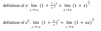
ln(x)

the integral of 1 over x dx from 1 to x where x > 0

product rule for 3 or more

if y = f g h, then y’ = f’ gh + g’ fh + h’ * fg 

derivative of inverse formula

g’(c) = 1 over f’(g(c)) where f is original function and inverse function is g

riemann sums

• riemann sum: b-a over n times (f(a) + f(a+a)... + f(b-1) + f(b))

• riemann sums underestimate when concave up and overestimate when concave down (same as LE) 

trapezoidal rule

• trapezoidal rule: 1/2 times b-a over n times (f(a) + 2f(a+1)... + 2f(b-1) + f(b))

• trapezoidal rule with different intervals: just make trapezoids (you can still factor out 1/2 to make it easier 

simpsons rule

• simpsons rule: 1/3 times b-a over n times (f(a) + 4f(a+1) + 2f(a+2)... + 4f(b-1) + f(b))

• for simpson’s rule, the num of intervals has to be even and at least 4 

LE underestimation

• f(x) is concave up 

• error is positive

LE overestimation

• f(x) is concave down 

• error is negative

LE function vs estimator

• f(x) vs y 

• delta f is f(x) - f(c) 

• delta y is dy 

• delta y is f’(c) times dx, because dy/dy equals slope at c 

• delta f is the difference in f(x) values on f(x) at x vs c 

• delta y is the difference in y value on the linear estimator at x vs c 

• error is delta f minus delta y

parametrics horizontal and vertical tangents

horizontal tangents (follows same rule as slope)

• dy/dt = 0 and dx/dt does not equal 0 

vertical tangents (follows same rule as slope)

• dy/dt does not equal 0 and dx/dt = 0

parametrics second derivative formula

x’y’’ -x’’y’ over x’ cubed

symmetric difference quotients

this is just when you take the next xy pair and the previous xy pair and find the slope, so that the xy pair in the middle has about the same slope

implicit differentiation

to do this, just take derivatives of both sides. remember y is a function (like u) so the end of chain rule is always y’. you are solving for y’ in terms of x and y.

implicit differentiation horizontal and vertical tangents

horizontal tangents (follows same rule as slope)

• numerator = 0, denominator does not

vertical tangents (follows same rule as slope)

• numerator does not equal 0, denominator = 0

implicit differentiation second derivative

take the derivative of y’ and then replace y’ with what it equals.

remember if smt is differentiable, it has to be continuous, but just bc something is continuous, does not mean it is differentiable (cusp) 

ok

when are you speeding up/slowing down

if velocity and accel have same sign, speeding up

if diff signs, slowing down

solids of revolution problems

• identify area of region (one function minus another)

• identify if you subtracted right minus left, use dy, if you subtracted top minus bottom, use dx 

• set up an equation using pi r squared h or pi R squared minus r squared h where h is dy or dx and r is one function minus another 

• if using dy, you have to transform equation so that it is in terms of y 

• if in terms of x, integral is from x1 to x2 of points of intersection and if in terms of y, integral is from y1 to y2 of points of intersection 

• if you have calc, don’t simplify cuz you’ll just make algebra mistakes; plug into calc integral function 

• remember to distribute square to all parts of r

• solve

FTC problems

when doing FTC, always remember to just do g(b) - g(a) even when a is 0 and you think you won’t need it, because a lot of times a value of x actually has a nonzero  value when put in the function

finding delta from epsilon algebraically

• you go from L - E < f(x) < L + E to the form c - delta < x < c + delta 

• simplify until you have c minus a value, x by itself, and c plus a value 

• if 2 delta’s, choose smaller

critical points of f(x)

values where f’(x) = 0 or is undefined

binomial expansion derivative practice

• do product rule and REMEMBER TO CHAIN RULE FULLY 

• factor out greatest common factors (coefficient and exponent - 1 of each binomial factor) 

• combine like terms 

• you can also do using ln, but it lowkey takes more time: 

  • put each side to the ln and separate right side using log multiplication rule 

  • bring down power from logs 

  • differentiate using chain rule on right, implicit on left 

  • multiply y (original function) to right hand side so you’re solved for y’ 

  • simplify

parametrics practice

• to convert to cartesian, you can solve for t in terms of y and sub in to x but usually you have to find some clever way to do it. if it’s an ellipse, know that you have to manipulate using sin squared + cos squared equals 1. 

• to find dy/dx at a point, take dy/dt and dx/dt and divide those

norm of partition

partition with greatest width

k, n, for loop problems

• set x = k/n or some multiple 

• dx is b-a over n 

• find the limit of x as n approaches infinity of the upper and lower bound (b and a) 

• substitute in to find dx 

• rewrite the function, substituting in values for a, b, k/n, and dx 

symmetric limits

the integral of an odd function from an evenly spaced integral on both sides of 0 is 0, and an even function is 2 times the integral from 0 to whatever number

dv of annuli

pi times R squared minus r squared times dx

trig derivatives

sin(x)	cos(x)
cos(x)	-sin(x)
tan(x)	sec²(x)
csc(x)	-csc(x)cot(x)
sec(x)	sec(x)tan(x)
cot(x)	-csc²(x)

trig function integrals

sin(x)	-cos(x)+c
cos(x)	sin(x)+c
tan(x)	ln|sec(x)|+c
csc(x)	-ln|csc(x)+cot(x)|+c
sec(x)	ln|sec(x)+tan(x)|+c
cot(x)	-ln|csc(x)|+c

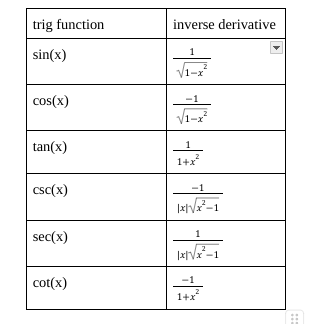
trig function inverse derivatives

derivative and integral of b^x

derivative: ln(b) times b to the x

integral: 1 over ln(b) times b to the x + c

derivative and integral of 1 over x

derivative: -x^-2

integral: ln|x| + c

reversal of bounds on limits of integration

just put negative in front

how to determine if the inverse of a function is a function

- it has to be continuous (poly or given).

- take the derivative and plug in end points, or graph, or in some way confirm that the derivative is always positive or always negative. this confirms that f(x) is strictly increasing or decreasing. for example, if the derivative is the function 9x^2 + 2, you know it’s always positive because you can graph it and see.

how to take derivative of inverse

• first prove inverse is a function

• then use inverse function: 1 / f’(g( c ))

process for 2nd derivative of parametrics

ddt of dy/dx over dx/dt

property of Riemann sums

if f is integrable on [a,b] and Rn is a riemann sum, then the limit of Rn as n approaches infinity equals the integrand f(x) dx from a to b

infinite Riemann sums limit

limit as n approaches infinity of Rn equals the limit as n approaches infinity of the summation from k=1 to n of f(ck) times delta x k

how to do ferris wheel problem

• formula: A(sin(B(x-C))) + D

• A is amplitude, how much it changes from midline

• B is 2 pi over period, always going to have pi on top so it’s 2 pi divided by the amount of time it takes to get back to one point

• C is how much left/right so base it off of max or mid of sin or cos

• D is how much midline is shifted up from ground

• REMEMBER that B value is OUTSIDE parenthesis so you have to distribute

• distribute so that you can put in calculator

• minus shifts right (remember algebra II)

trapezoidal is backwards in what way

concave up is overestimating and concave down is underestimating