case of the missing population variance

sampling distribution of s

distribution of s is skewed, in larger N, it will look more normal and vary less from σ; in smaller N, it will look less normal, vary more from σ

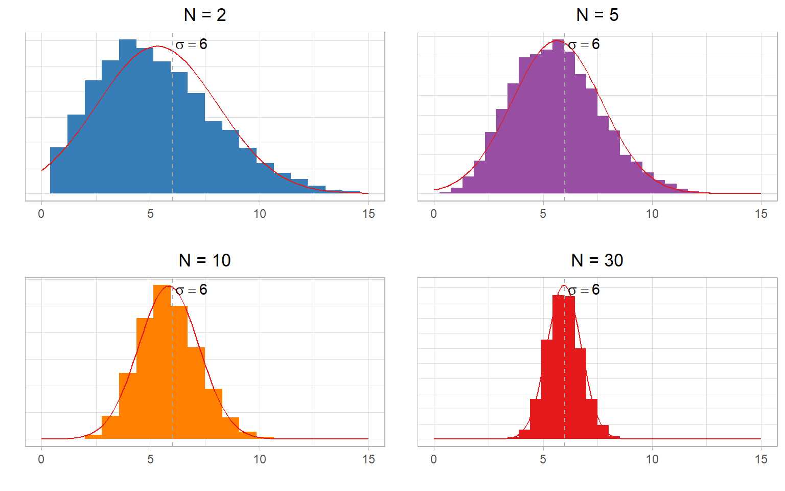
when we don’t know σ. why can’t you find SE of the (normal) sampling distribution of means using SE = s/√N

when sample size is small, the distribution will have fatter tail —> a larger proportion of sample means would be counted as extreme values than we expect

more likely to make Type I error (false rejection)

william gosset

• worked at Guinness Brewing Company, did small-sample experiments in which he changed the ingredients in the beer recipe

• published papers under the pseudonym “student” to avoid angering his employer

• most famoous for discovering the t-distribution which accounts for the added uncertainty due to sampling variation in s

how does the t-distribution account for added uncertainty due to sampling variation in s

adds an extra parameter: df, number of data points that can freely vary after accounting for estimated values

larger df: thinner tails, more similar to normal distribution

smaller df: fatter tails, less similar to normal distribution

• fatter tails —> we need to move more SE away from the mean to include 95% of the dsitribution in the center

calculate the t-statistic (one sample t-test)

t = (x̄-μ₀)/s_x̄

where s_x̄ = s/√N

df = N - 1

assumptions of a t-test

• the sampling distribution follows a normal distribution

• the observations are independent

• there are no outliers (influential data points not from our population, we have reason to believe they’re from a different population- not just because they stand out)

• sampling was random

numerical and normality checks

• skewness and kurtosis (both = 0 in norm dist)

• Kolmogorov-Smirnov (KS) test, Shapiro-Wilk test

Kolmogorov-Smirnov (KS) test, Shapiro-Wilk test

hypothesis tests of whether sample distribution is significantly different from a (population) normal distribution (null hypothesis = normality)

sensitive to N, tend to always reject if N is big

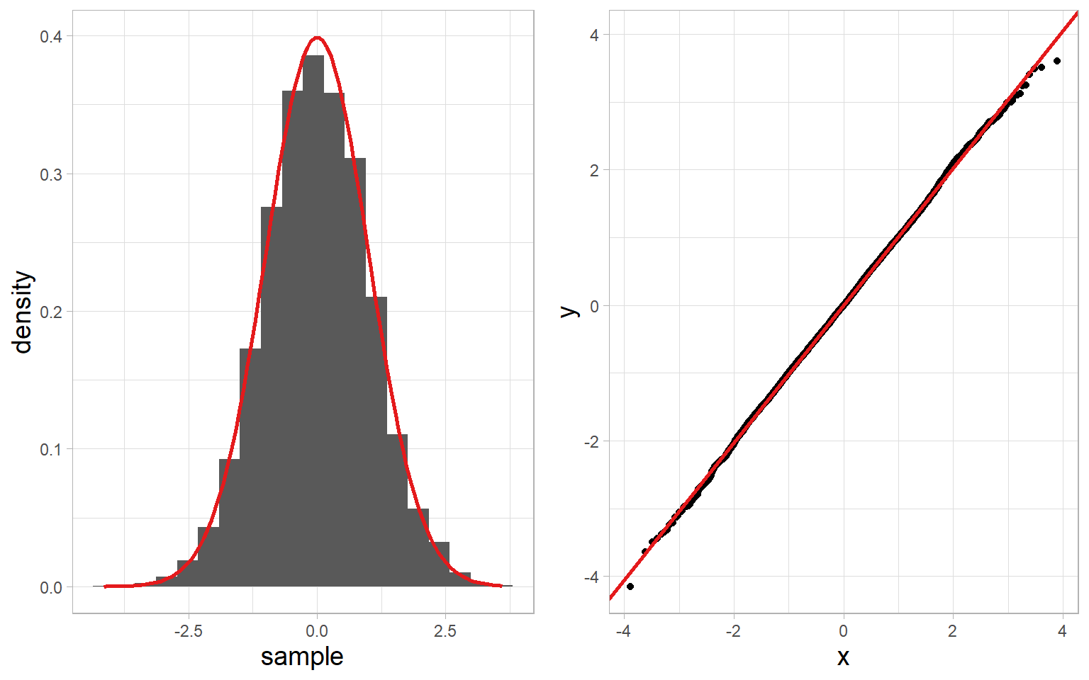
graphical normality checks

histograms/density plots

quantile-quantile (Q-Q) plots

Q-Q plot

x-axis: theoretical quantiles of the normal distribution

y-axis: quantiles of the data

if normal, points should fall in a straight line

confidence interval

interval estimate

range for which any random sample from the population will contain μ with probability 1 - α

calculate confidence interval

x̄ ± critical value*s_x̄

find the critical values: the values on the distribution such that 2.5% is in the left and right tail for α = .05

turn the critical values onto the scale of the original variable with sample mean and SE

paired samples t-test

t-test that builds in a dependence structure:

• variable measured at two points in time for the same N persons

• variable measured for pairs of subjects (younger/older siblings, husband/wife pairs)

take the difference score (D) for each pair of observations

nil hypothesis

setting a null hypothesis to a difference of zero

a way to determine test for differences in general

paired t-test statistic

t_D = (D - μ₀)/(s_D/√N) with df = N - 1

N is the number of pairs

average difference divided by SE of difference scores (μ₀ often 0)

independent groups

testing whether two independently sampled groups have the same population mean

randomized experiments where different groups get different treatments

difference in pre-existing groups

independent samples t-test assumptions

normality of sampling distributions, independence of observations, no outliers, random sampling PLUS

homogeneity of variance: even if the populations have different means, they have the same SD around those means

pooled variance

to get the best estimate of the shared population variance, we need to pool them

weighted average of the two sample variance

independent samples t statistic

t_x̄1-x̄2 = (x̄1 - x̄2)/(s_x̄1-x̄2)

s_x̄1-x̄2 = pooled standard error = s_p*√(1/n₁ + 1/n₂)

df = n₁ +n₂ - 2

Welch-Satterthwaite correction

same test statistic as before, but the SE doesn’t pool variances (s_{x̄1-x̄2 =} √((s²₁/n₁) + (s²₂/n₂)) and modifies the degrees of freedom to make them smaller than (n1+n2-2)

default in R, helps if homogeneity of variance doesn’t hold