biostats - unit 1

console

stat output and successful code show up here

script (.rmd)

type codes here

viewer

graphs and help files show up here

environment

what I told R to plan to use today (objects, variables, models, etc. are stored here)

vector

set of numbers

creating a vector with 5 numbers: c(96, 95, 99, 97, 98, 96)

assign to a variable by: tempF ← c(96, 95, 99, 97, 98, 96)

goal of biostatistics

focuses on collecting, describing, and drawing conclusions from data to learn more about the world

uses estimation to infer an unknown of a population using sample data

data

cumulative measurements of individual biological entities

population

all individuals or observations in the world (group we are typing to gain info about)

sample

subset of measurements we collect and analyze to learn about the population (what we measure to draw inferences)

parameters

describe populations (true value)

• fixed and constant

  • represented by mu

estimate/statistic

taken from samples

• random, change with each sample

  • represented by capital Y with a bar on top

descriptive statistics

implies that statistics is an estimate of parameter

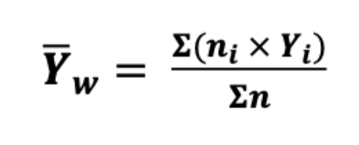
weighted mean

assigns different importance (weights) to each data points so it reflects relative importance in overall calculation

statistics of locatoin/central tendency

mean, median, mode

mean vs median

mean = mathematical center of gravity, median = average individual (middle measurement)

statistics of dispersion

range, IQR, variance, standard deviation, coefficient of variation

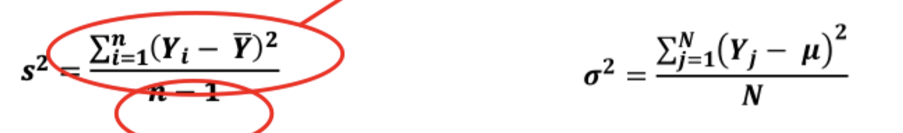
variance

expected squared difference between observations and the mean

• estimate = s²

  • denominator is n-1 for degrees of freedom

• parameter = lowercase sigma²

  • denominator is just N

standard deviation

measure of dispersion that weighs each item by distance from mean

• estimate = s (sqrt of variance)

  • parameter = lowercase sigma (sqrt of variance)

coefficient of variation

standard deviation expressed as percent of mean

• CV = sample standard deviation (s) / Y (sample mean) x 100

when to use variance

understand how much values in a dataset vary from each other

when to use standard deviation

understand how data points typically deviate from the mean

when to use coefficient of variation

used to compare variation between two datasets

inference

requires independent and random sampling

sampling bias

systematic difference between estimates and parameters

• samples aren’t representative of population

sampling error

undirected deviation of estimates away from parameters

• influenced by chance and differs among samples from the same population

  • decreases with increasing sampling size

sampling distribution

probability distribution of all possible sample means

• random process

• sample from a population provides an estimate of the parameter

sampling error

difference between parameter and estimate

key features of sampling distribution

• normally distributed

• mean of sampling distribution = true mean of population

• spread depends on sample size used for estimate

  • as sampling size increases, parameter estimates become more precise and spread of sampling distribution decreases

standard error

standard deviation of an estimate’s sampling distribution

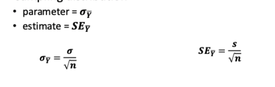
key features of standard error

• decreases with increasing sample size

• tells us how close sample mean is to true mean (population)

• tells us how unusual a sample is

standard error vs standard deviation

SD describes how individuals in a sample differ from sample mean

SE describes how far sample mean is from true mean

95% CI

range of data around potential sample mean values in our sampling distribution for which we are 95% sure contains the true population parameter (2 * SE)

addition rule for probability

if two events are mutually exclusive, then P[A or B] = Pr[A] + Pr[B]

multiplication rule for probability

if two events are independent, then P[A and B] = Pr[A] x Pr[B]

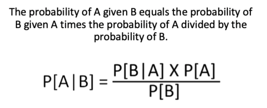
Bayes Theorem

use for conditional probability

variable

any characteristic that varies from one biological entity to another

categorical variables

qualitative characteristics of individuals that do not have a numerical magnitude

• nominal = unordered descriptions

• ordinal = ordered descriptions (1-5 how are you feeling, etc.)

• binary = 2 mutually exclusive outcomes (yes or no)

numerical variables

quantitative measurements of individuals that have a numerical magnitude

• continuous = measured data, can have infinite values within possible range (decimals, fractions, etc.)

• discrete = observations can only exist at limited values, often counts (whole numbers)

tidy data

standard way of mapping the meaning of a dataset to its structure

• variable = column

• observation = row

• cell = single measurement

visualizing one variable categorical data

• frequency table = counts of the number of occurrences of each category

• bar graph = frequency distributions of categorical data

one variable numerical data

goal = measure center, spread, and shape of data

• frequency table = counts the number of occurrences within set bins

• histogram = displays the frequency distributions of numerical data

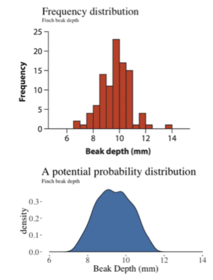
frequency distribution vs probability distribution

frequency distribution = describes the number of times a value occurs in a sample

probability distribution = describes the proportion of the population with a value

when is an estimate considered to be unbiased

when across infinite repeated samples, the average of the estimates equals the true parameter value