Biostats Final

Why do we collect data?

To answer if variability is real or not

Systematic error

The error only goes towards one direction

• Ex: If we are measuring weight with an uncalibrated scale, it will add or reduce the weight systematically

Random error

Due to chance, the error can go into both directions

• Ex: If we take two samples of the class and measure your weight, the difference can vary for both directions

Quantitative data

Numeric

Qualitative data

Categorical

Types of quantitative data

Continuous

Discrete

Types of qualitative data

Binary

Nominal

Ordinal

Continuous variables

Variables that describe the values of a continuous scale

• Ex: weight, BMI, height

Discrete variable

Variable that describea the values of finite events, usually based on whole numbers

• Ex: number of siblings, age…

Binary variable

Variable that describe the values of any event that only has two categories

• Ex: death (yes, no), physically active (active, non-active)

Nominal variable

Variable that describes the values of any event that has two or more categories without order

Ex: who are the people that live with you? (live alone, partner, friend, family…), NBA team (Lakers, Bulls….)

Ordinal variable

Variable that describe the values of any event that has two or more categories with an order

Ex: grade in the course (A,B,C…), BMI (normal, overweight, obese…)

Mean (central tendency)

sum of the values of one variable, divided by the number of values

Median

A central tendency estimate that is exactly in the middle of the sample, dividing the sample in half

• Can be used to address outlier issues

  • Equation: Even numbers: Average of n/2 and (n+2)/2

  • Odd numbers: (n+1)/2

Variability measures

Min and Max values (amplitude)

Position measures

Variance

Standard deviation

Coefficient of variation

Standard error

Min and Max values (range)

The difference between the extreme values

Position measures

Measures that separate the observations in equal parts (or almost), like the median

• Ex 1: Quintiles

  • 1 (20%), 2 (20%), 3 (20%), 4 (20%), 5 (20%)

• Ex 2: Percentiles

  • P10 (10%), P5 (5%), P50 (50%)

Variance

An average of the difference (squared) of each observation in relation to the overall mean

• Squared because the differences can have negative values

• Result doesn’t have the same unit as the individual values or the mean

Standard deviation

Square root of the variance

• How much, in average, each value is to the mean

• Uses the same unit as the original variable

Standard Error

Shows how much the sample mean is likely to vary from the population mean due to random error or sampling

• Smaller SE suggests a more accurate representation of the population mean, while a larger SE indicates more uncertainty

Variation coefficient

(Standard deviation/mean)*100

• The ratio of the standard deviation to the mean, often expressed as a percentage

• Allows for comparisons between data sets with different means or units

Interquartile range

Range based on the 25th percentile and 75th percentile

What can we use categorical variables to measure?

Frequency

• Count, raw number of events

Probability

• The portion of the number of events compared to the sample

  • % of individuals with cancer

Odds

• Chance

• Comparison of individuals

  • Odds of having cancer compared to not having cancer

Probability

number of favorable outcomes/ number of possible outcomes

multiplicative rule for probability

used for the probability of the occurrence of both of two events, A and B

• Prob(A and B)= Prob(A) x Prob (B)

Additive rule for probability

used for the occurrence of at least one of event A or event B (either)

• Prob(A and B)= Prob (A) + Prob(B)-Prob(A+B)

Odds

Considers the probability of a successful event compared to a probability of a failure/unsuccessful event

• Can present values from 0-infinity (not percentage)

Prevalence

represents the burden of disease in a particular time

• number of people with the disease at particular point in time/total population

Incidence

represents the burden of new cases from a disease

risk=cumulative incidence= number of new cases of disease in period/number initially disease-free

Normal distribution

Used for continuous variables

Symmetrical around the mean

Bell-shaped

Describes biological events well

Values in the middle of the distribution are more frequent

Is tall and narrow when the standard deviation is low

Short and wide for higher standard deviation

central limit theory

Principle that the distribution of sample means approximates a normal distribution as the sample size gets larger, regardless of the population’s distribution

parameters to know if the distribution is normal

skewness

kurtosis

statistical test

visual interpretation

skewness

a measure of lack of symmetry. values close to 0 indicate normal distribution, or symmetry

kurtosis

a measure that describes how heavily the tails of a distribution differ from the tails of a normal distribution

• values close to 3 indicate normal distribution

What is the problem if the distribution is not normal?

Can’t use MEAN as the central tendency measure, because it will be biased, instead we must:

• must use other measures like MEDIAN

• categorize the variable

• make a transformation

Correlation

relationship between two numeric variables

measures the degree in which the variables are related

coefficient values ( r ) range btw -1 to 1

• -1: perfect negative correlation

• 0: no correlation

• 1: perfect positive correlation

R squared

Indicates the percentage of the variability of the outcome that is explained by the exposure

Pearson correlation test

used for continuous variables

at least one should have a normal distribution

Spearman correlation test

based on ranks

continuous or ordinal variables

used when we don’t have normal distributions

null hypothesis

hypothesis that there is no significant difference btw specified populations, and any observed difference is due to chance or error

• Example when looking at mean physical activity btw English and Spanish speakers

  • mean physical activity is NOT different

alternative hypothesis

there is a significant difference btw the specified populations

• Example when looking at mean physical activity btw English and Spanish speakers

  • mean physical activity is differnt

Type 1 Hypothesis Error

Rejects the null hypothesis, when the null hypothesis is TRUE

Says there’s a difference when in fact it hasn’t

P-value (5% or <0.05)

Type II Error

Don’t reject the null hypothesis, when the null hypothesis is FALSE

Don’t say there’s a difference when in fact there is a difference

Confidence interval

Represents the variability of our measure, based on a sampling distribution

• Usually we use 95%

ANOVA

association of a numeric exposure with a categorical exposure with TWO OR MORE categories

based on independent samples

T-test

numeric outcome, binary exposure

comparison of means btw TWO INDEPENDENT groups

• example: comparing if the mean physical activity is the same in males and females

Paired sample

Either same individuals with two measures over time or

pair of individuals, with each having one measure

Types of categorical variables

Dichotomic (two categories)

Politomic (three or more categories)

Ordinal (categories have a specific order)

Use 2×2 tables

Chi-squared

Fisher Exact

McNemar Test

Use 2xK Tables

Chi-squared

Linear trend

2×2 contingency table

Longitudinal estimation: Incidence/Prevalence

ICexp=a/m1

ICnexp=b/m2

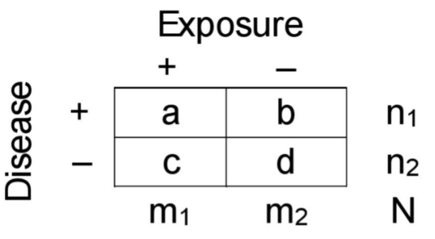
Longitudinal estimation: Odds

ODDSexp= a/c

ODDSnexp= b/d

Case-control estimations: Exposure prevalence

PRexp=a/n1

PRnexp=c/n2

Case-control estimations: Odds

ODDSexp=a/b

ODDSnexp=c/d

Chi-squared test

Compares the observed values in each of the categories of the table with the expected values

Degrees of freedom

An estimation of the number of independent categories in a particular statistical test

Fisher Exact Test

Used when the chi-squared approximation is not good

Used when expected values are too small

• Total N<20, independent of the expected values

• Total N btw 20 and 40, with expected values <5

Computationally “heavy”

Uses the exact probabilities of the hypergeometric distribution

Difference btw correlation and regression

With correlation we can only see how much two variables are related to each other

• Correlation of 0.80 means that two variables are positively and strongly correlated

With the regression model, we can estimate how much one variable is affecting the other

• A regression coefficient of 2.0 means that, on average, each unit increases in the exposure increases 2.0 units in the outcome

Residual

the error btw the observed values and the estimate values based on the regression