Financial econometrics - terminology

cash

• represents a claim on the stream of services that it can secure by virtue of its roles as a medium of exchange

fixed-income securities

• provide two sources of return:

• a stream of interest payments (or coupons) that are made at fixed, regular intervals

• the eventual return of principal at maturity

• distinguishing feature: the periodic payment is known in advance

• short-term assets whose markets are particularly active/liquid are known as money market fixed-income securities, eg treasury bills and eurodollar deposits

derivative securities

• provide a payoff based on the value(s) of other assets such as commodities, bonds, or stocks

• eg options and futures

options

• the right to do so (not obliged) to buy or sell

• offer the buyer the right (not the obligation) to buy (call) or sell (put) the underlying asset at a particular price during a certain period of time or on a specific date

futures

• obligation to buy/sell at a future date

• specify the delivery of either an asset or a cash value at a time known as the maturity for an agreed price, which is payable at maturity

equity securities

• equities/common stock give the owner an equity stake in a company and a corresponding claim on company assets and earnings

bid

• the highest price a buyer is willing to pay

ask

• the lowest price a seller is willing to sell

market capitalisation

• share price multiplied by the volume of outstanding shares

volume in box

• volume of trade on that particular trade

• not used in market capitalisation

stock market index

• a summary measure of how well the stock market is doing as a whole

• indices create portfolios by putting together a large group of stocks in a certain way

• the index shows how much the portfolio is worth

• expressed in terms of an average price that has been normalised in some way

• over 1700 companies trading in London Exchange as of 2024

price-weighted index

• the weight given to each stock is the price of the share

• sum up the price of one share of each company gives the base for price-weighted index

value-weighted index

• the weight given to each stock is proportional to the total market capitalisation

• sum up the market capitalisation of all the companies gives the base for the value-weighted index

stylised facts

• commonly observed patterns

integrated process

• nonconstant mean and variance

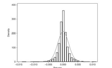
leptokurtic distribution

• a sharp peak in the centre of the distribution

• slightly heavier tails

• there are many observations where the exchange rate hardly moves and for which there are a greater number of smaller returns than there would be if returns were randomly drawn from a normal population

• common in exchange, equity, and commodity markets

platykurtic distribution

• lower peak and lighter tails than a normal distribution

moment

• a snapshot of the shape of the distribution

volatility

• how often the return deviates from the average return and how far it deviates

• measures how risky an investment is

• if volatility is high, then asset prices are changing more rapidly when volatility is low

• the volatility of an asset can be measured by the standard deviation of its returns

sample covariance

• a measure of co-movements between the returns on two assets

• a positive covariance signifies that the returns of the assets move together

• a negative covariance signifies that the returns of the assets move in opposite directions

percentile

• a measure that indicates the value below which a given percentage of observations in the sample fall

• for instance, the median, or the 50th percentile, has 50% of the observations below it

• a set of statistics that summarize both the location and the spread of a distribution

inter-quartile range

• the difference between the 25th percentile (first quartile) and the 75th percentile (third quartile)

• provides an alternative to the standard deviation or variance as a measure of the dispersion of the distribution

value at risk (VaR)

• quantifies the loss that a bank can face on its trading portfolio within a given period and for a given confidence interval

• at a given level of confidence, VaR is the worst loss that won’t be exceeded over a certain period of time (typically one day)

• 1st and 5th percentiles are important when calculating this

• quoted as a positive number

• defined in terms of the lower tail of the distribution of trading revenues

autocorrelation

• the strength of association between the current return, rt, and the return on the same asset k periods earlier, rt-k

• used to test the predictability of returns

Efficient Market Hypothesis (EMH)

• the idea that the market cannot be ‘beaten’

autocorrelation in squared terms

• essentially the autocorrelation of the variance

• measures the correlation between the variance of returns at time t, and the variance of returns at time t-k

treasury bills

• simplest form of government debt

• the government sells treasury bills in the money market and redeems them at the maturity of the bill (around 3, 6, 9 months)

• no interest is payable during the life of the bill so they trade at discount to the face value of the bill that will be paid at maturity

eurodollar deposits

• deposits of US banks that are denominated in US$ but held with banks outside the US

• have relatively short maturity (<6 months)

• the eurodollar deposit rate is used as a representative short-term interest rate

bond market

• the place where longer term borrowing of governments or corporations is conducted

bond

• a security that promises to pay the owner of the bond its face value at the time of maturity of the bond and usually an ongoing coupon payment prior to maturity

• maturity can be as long as 30 years

zero-coupon bonds

• pay no regular interest and are traded at prices below their face value

stripping

• when zero-coupon bonds are created from coupon-paying bonds by separating the coupons from the principal and trading each of these components independently

long position

• the entity who commits to purchase the asset on delivery

short position

• the entity who commits to delivering the asset

risk-free rate

• interest rate on a government bond

• usually measured in annual rate so if calculating excess returns, need to ensure it is annualized

yield

• the yield on a bond is the discount rate that equates the present value of the bond’s face value to its price

term structure

• the relationship between time to maturity and yield to maturity

yield curve

• a plot of the term structure of yield to maturity against time to maturity at a specific time

sample variance

• a measure of the deviation of the actual return on an asset around its mean

sample standard deviation

• a measure of the riskiness of an investment (volatility)

sample kurtosis

• if there are extreme returns relative to a benchmark distribution

• K>3 = more extreme returns in the data (heavier tails)

capital asset pricing model (CAPM)

• a way of relating the risk of an asset to market risk

excess return

• the return on asset i relative to risk-free rate rft

• r_it - r_ft

systematic risk

• risk inherent to the entire market

• nondiversifiable

• market risk

• this caused rhe 2008 financial crisis as firms could not change the equilibrium

idiosyncratic risk

• diversifiable

• asset-specific risk

white noise

• a series that satisfies these conditions

• means we have zero mean, homoskedastic variance, and zero autocorrelation

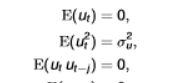
homoskedasticity

• variance of ut is constant over time

objective function

• a function we would like to miminise/maximise the function

• we would like to reach that function

identity matrix

• matrix in its inverse multiplied by the matrix itself

• results in a matrix with ones in the diagonal and zeros elsewhere

• has the nice property of leaving a vector unchanged

• why it is called identity (keeps the identity of the vector)

Fama-French 3 factor model

• Fama and French proposed to augment the VAPM model by including two additional risk factors to explain investment returns

• these factors are referred to as size and value

size/small minus big (SMB) factor

• accounts for the spread in returns between small- and large-sized firms

• size is determined by market capitalisation = share price * number of shares outstanding

• the performance of small stocks relative to big stocks

• a risk factor to explain the return on a risky investment

value/high-minus-low (HML) factor

• an additional factor that captures the performance of ‘value’ stocks relative to growth stocks

• historic excess returns of (value stocks-growth stocks)

• we average across the year

• a risk factor to explain the return on a risky investment

value stocks

• companies with high book-to-market ratios

• the market is undervaluing the compnay

growth stocks

• companies with low book-to-market ratios

• the market is placing a high premium on expected future earnings or growth potential

book-to-market ratio

• book value of firm

• historical cost or accounting value/ market value of firm (market capitalisation

coefficient of determination (r-squared)

• a natural measure of the success of an estimated model

• it is the proportion of the variation in the dependent variable explained by the model

event analysis

• used in empirical finance to model the effects of qualitative changes on financial variables arising from a discrete event

• typical events that are relevant in finance arise from announcements such as the change in a company’s CEO, a monetary policy announcement, or dramatic new events

momentum factor

• captures the returns to a portfolio constructed by buying stocks with high returns over the past 3 to 12 months and selling stocks with lower returns over the same period

• captures the presence of herd behaviour among investors who are following market movements

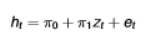
structural equation

• used in IV estimation

• describe some aspect of the ‘structure’ of the economy or market

• they carry behavioural content (eg how investors react to risk)

• they are typically of the greatest interest to the modeller

• they can contain one or more endogenous regressors, and cannot be consistently estimated by OLS

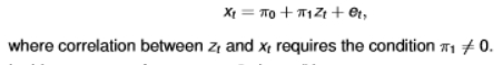
reduced form equation

• expresses an endogenous variable exclusively in terms of exogenous variables

• expresses an endogenous variable as a function of all of the exogenous and predetermined variables in the system

• reduced form equations can only contain exogenous variables on the RHS

• they can be consistently estimated by OLS

• typically do not carry any behavioural interpretations

• the estimated reduced form equation represents a weighted average of the exogenous and predetermined variables

• weights are determined optimally in the sense that the estimated equation provides the best predictor of the endogenous variable from a conditional expectations point of view

identified structural equation

• if there is at least one instrument for each endogenous variable

• L(instruments)=N(endogenous regressors)

unidentified structural equation

• the parameters of an unidentified equation cannot be consistently estimated

• L (instruments)< N(endogenous regressors)

overidentified structural equation

• L(instruments)>N(endogenous regressors)

relevant instrument

• an instrument that satisfies the exogeneity condition

• if this condition is not satisfied and the coefficient equals 0, the link between the two variables is broken

• this means the instrument carries no information about the endogenous regressor xt

weak instrument

• where the instrument does exhibit some correlation with xt but the correlation is relatively low

• for example, if the coefficient was 0.001, we would have a problem

• if the coefficient is small, then most of the information will translate intp et

• this results in loss of information in et

endogenous variables

• regressors that are correlated with the disturbance term

exogenous variables

• regressors that are uncorrelated with the disturbance term

endogeneity problem

• violation of the no-correlation assumption

endogeneity testing

• testing a regressor for possible correlation with the disturbance term

reduced rank test

• extension of testing framework for weak instruments, where there are N endogenous variables, L instruments, and K exogenous variables

• based on a joint test of the quality of all possible instruments for the full set of endogenous regressors

valid instrument

• satisfies the exogeneity condition and in the reduced form regression, the coefficient on the instrument does not equal zero

• even though its value may be small so that weakness in this instrument is not precluded

• can do robust testing despite this

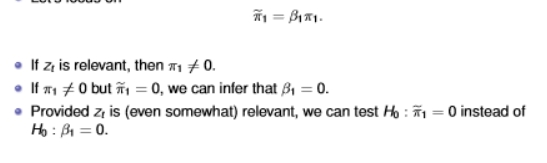
anderson-rubin test

• a t/F test of the null hypothesis

• a condition that applies if zt is a valid instrument for xt and the relevance condition is met

• if the hypothesis cannot be rejected, then B1 = 0 also can’t be rejected

• weak instruments imply that π1 is small so that B1π1 is also small, also provided that B1 itself is not too large

• if B1 is large, B1 will diverge substantially from its value under the nul hypothesis B1=0

tobin Q’s

• the ratio of the market value of a company to the replacement cost of its assets

• the logarithm of this can be used as a measure of firm performance

covariance stationary

• a time series is said to be covariance stationary, if the mean, variance, and autocovariances all remain invariant to the time periods in which they are calculated

• important as it allows us to build standard models and use the past behaviour of variables to extrapolate their behaviour in the future

• requires that all joint distributions of the time series remain unchanged when shifted over time

• it fails when the mean has a time trend, or when the variance is time varying

partial autocorrelation function (PACF) at lag k

• measures the relationship between yt and yt-k

• now the intermediate lags are included in the regression model, so that their effects are controlled for

• another measure of the dynamic properties of AR models

vector autoregressive model (VAR)

• with a multiply equation system where each variable is dependent on its own lags and the lags of all other variables

• the assumption of covariance stationarity of all the variables is maintained

Granger causality

• based on the presence/absence of predictability

• does not of itself signify causal influence

• Granger causality is a statistical concept used to determine whether past values of one time series help predict the current or future values of another time series, beyond what is possible using the past values of the dependent variable alone

granger causality testing

• one method of identifying the system dynamic of a VAR and verifying block significance, thereby enhancing our understanding of variable interactions over time

impulse response analysis

• used to examine system dynamics

• focuses on impulse responses by tracking the transmission effects of shocks to the system on the dependent variables

shock

• something happening to et that can’t be explained by y1, y2, y3

variance decomposition

• we decompose the forecast variance into relative effects, expressed as percentages of the overall movement

• in the case of the SVAR model of equities and dividends, the approach is to express the forecast error variances of equities and dividends in terms of the structural shocks v1 and v2

scalar (one variable) dynamic model

• a single dependent financial variable is explained using its own past history as well as lags of other relevant financial variables

structural VAR models

• allow for contemporeaneous interactive effects among the variables

• an important characteristic for VAR is that each variable in the system is expressed as a linear function of its own lags as well as the lags of all of the other variables in the system

mean aversion in returns

• exhibiting positive autocorrelations

mean reversion in returns

• exhibiting negative autocorrelations

structural VAR

• the disturbances v1t and v2t represent structural disturbances or primitive shocks that are uncorrelated E(v1t, v2t) = 0

• this system can be used to construct impulse responses for ret and rdt, with respect to the structural shocks v1t and v2t

• as the SVAR model is dynamic, the shocks have a contemporaneous effect as well as a dynamic effect

nonstationary time series

• time series that exhibit strong evidence of trends over long periods of time - important property of asset prices

• trend behaviour often manifests in a tendency for a time series to drift over time in such a way that no fixed mean value is revealed

• this long term time trend is coupled with extended sub-periods in which prices wander above and below the trend line

• may embody both a deterministic trend or a stochastic trend

order of integration

• the process becomes stationary once differenced ‘d’ times

• a process is integrated of order d, denoted by I(d), if it can be rendered stationary by differencing d times

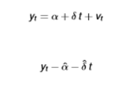
trend-stationary

• if de-trended yt is stationary

• vt is stationary

• most common is a linear trend but doesn’t have to be → d1t + d2²t

cointegration

• the ability to generate stationary time series as a linear combination of nonstationary time series

• occurs when two or more non-stationary time series are linked by a stable, long-run equilibrium relationship such that a linear combination of them is stationary

• implies that while the series themselves may individually exhibit stochastic trends, they do not drift apart indefinitely

cointegrating parameters

• the weights applied to each of the series in the combination

• the convergence of the cointegrating parameters are faster than the stationary parameters

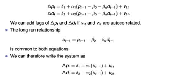
error correction model

• system behaves in such a way as to correct the equilibrium errors, ut-1

impulse response analysis

• in VAR or VECM, an impulse is like a sudden, unexpected shock

• eg a sudden increase in interest rates

• we are able to trace out how that shock affects each variable in the system over time

• it helps us to understand causal dynamics - who influences whom and for how long

• it can show whether a shock has temporary or permanent effects

variance decomposition

• how much of the total forecast error (uncertainty) in each variable is due to shocks in itself vs shocks in other variables

• ie, it splits up the forecast error variance into portions attributable to different shocks

deterministic trend

• manifests in exponential growth path

stochastic process trend

• arises from the accumulation of random forces that drive prices to wander above and below the path of the deterministic drift

stochastic trend component

• aggregates (or integrates) up the component shocks vj

spurious regression problem

• arises when two or more non-stationary time series are regressed on each other, leading to misleading high statistical significance, even when no real relationship exists

• when variables are integrated of order one but not cointegrated, the standard OLS produces high r-squared values, significant t-statistics, standard tests may appear valid (even though they are not as they violate stationarity and no serial correlation assumptions)

• in order to avoid the problem, the time series should be differenced

• regression of two I(1) series may show high r-squared and t-stats, even when uncorrelated

forecast

• a quantitative estimate about the most likely future value of a particular variable

• typically based on past information and current information about the variable and other observable variables that are thought to be related to it

ex ante forecasts

• the entire sample {y1, y2, …, yT} is used to estimate the model

• the task is to forecast the variable y over the future horizon T+1 to T+H

• uses all the information up to today and uses this information to forecast for the future

• made before outcomes are known

• it is useful for decision-making, unlike ex post forecasting