Biostatistics Exam #3 Review

Which of the following regarding dummy variables are true?

• A dummy variable usually takes a finite number of value

• The value of a dummy variable indicates categories of interest.

For example given g categories, the number of dummy variables should be g-1 for a model containing an intercept

True

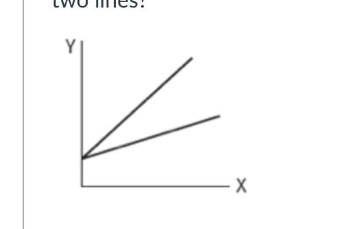
Please compare the following two lines. What is the relationship between these two lines?

Equal intercepts

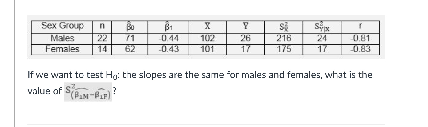
The following data involving regression of delinquency index (DI) (Y) on IQ (X). The sample of 22 observations consists of males only. Another sample of observations has obtained 14 females. The information needed to compare the straight line regression equations of males and females is given in the following table.

0.014

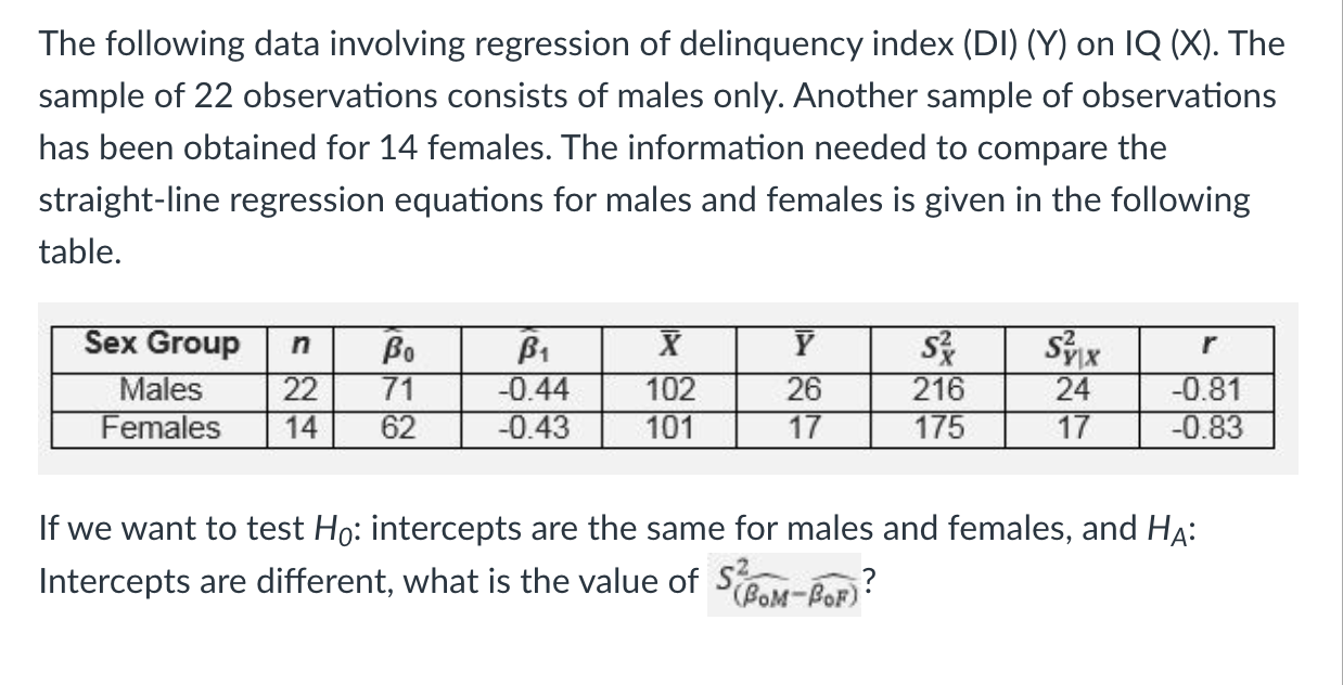
If we want to test H0: intercepts are the same for males and females and HA : intercepts are different what is the value

147.37

Multicollinearity can lead to

Inflation of variances of estimated regression coefficients

A measure of the effect of an unusual x value on regression results is called

Leverage

A large studentized residual value indicates an outlier with respect to

Both dependent and independent variables

Which of the following does not help detect violation of normality assumption?

Cook’s distance

Which of the following is a tool that detects an influential outlier?

DFFITS and Cook’s D.

As a first step of Forward stepwise regression procedure, what would you select as a candidate for the first addition is:

The X variable with the largest F* value

Which of the following steps are for the backward selection procedure?

Select with full model, repeat by deleting variable with the least significant F-test and then end with all variables have F-test p-value <alpha.

Which criterion is used to select the best regression model?

-Mallow’s Cp

-Adjusted R²p

-AlC

If you put too many variables into a regression model, including some unrelated to the outcome you are:

Overfitting

Which of the following is not one of the goals of model selection?

Multiple comparison

In a One-way anova, a factor refers to:

The independent variable

When a one-way analysis of variance is performed on samples drown from K populations, the mean square due to treatment (MSTR) is

SSTR/(K-1)

In ANOVA, a treatment refers to

A level of a factor

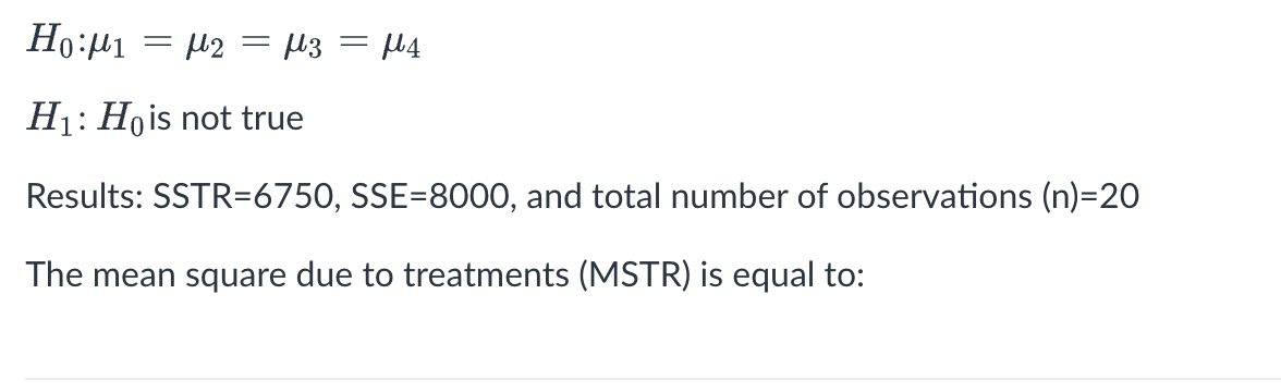
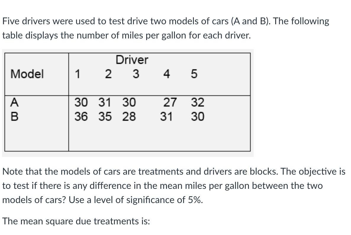
2250

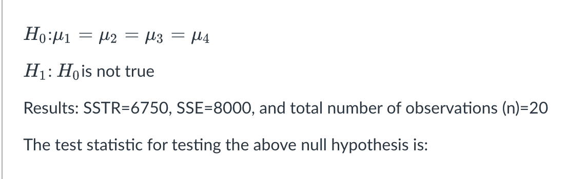
4.50

10

8

Fail to reject H0.

What is the Bonferroni procedure used for?

Protecting the experimentwise alpha error rate.

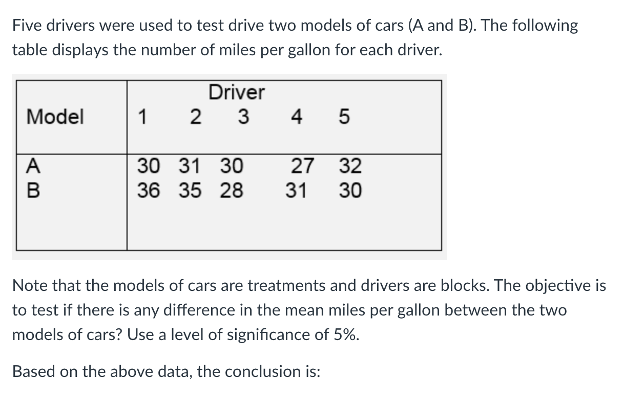
The principle of blocking in a randomized complete block design is:

To prevent confounding variables from obscuring the comparisons between treatment means.

Least square regression line

Y^= B0 +B1X

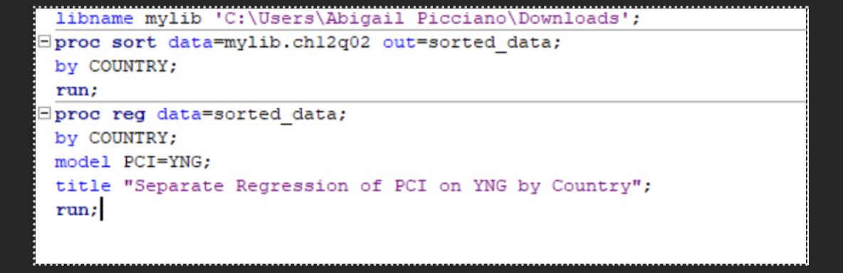
SAS code for lease square lines

Least square line equation

Y^=B0+B1X

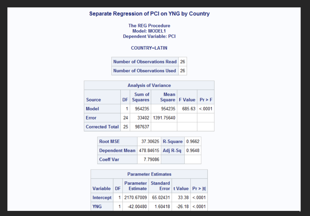
Least square line for Latin America

PCI^=2170.67-42.00X YNG

2170.67= intercept B0

-42.00= is the YNG B1 parameter estimate

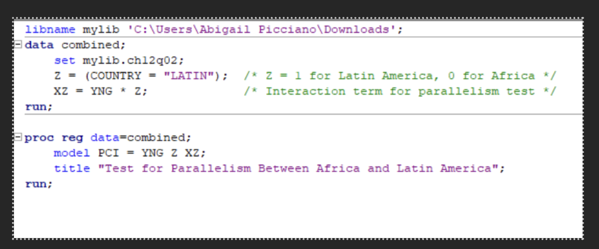
Parallelism tests of the slopes SAS code

Interpretation of parallelism

T p-value for XZ is <0.001 and would reject H0. Therefore, the regression lines AFRICAN and LATIN are not parallel; their slopes differ significantly.

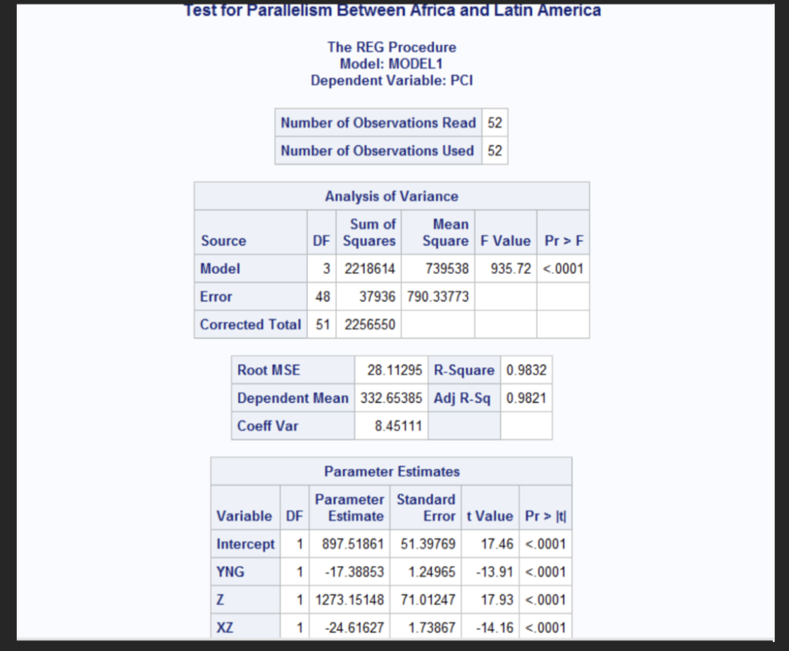
Test H0 the intercepts are the same for the countries versus HA the intercepts are different

The intercept estimate is B0= 897.52 which is the intercept for Africa and the coefficient for Z (B2) was 1273.15 with p-value <0.001 which indicates the intercept for Latin American countries differs from that of African countries meaning that is 1273.15 units higher than Africa when YNG is 0. When you add 1273.15 to 897.52 the estimate for the intercept for Latin America is 2710.67.

Test H0: The straight lines coincide for the African and Latin America countries. HA: The straight lines do not coincide

From the above output both the Z p value was <0.001 meaning the intercepts differ and the XZ p-value was <0.001 meaning the slopes differ and since both are significant H0 is rejected and the regression lines do not coincide the intercepts and slopes differ significantly.

Test H0: The population correlation coefficients are equal for the two groups of countries under study. Use alpha level of 0.05. Does your conclusion here class with your findings regarding the equality of slopes.

Z= ½ ln (1+(-0.983)/1-(-0.983)= ½ ln (0.017/ 1.983)= ½ ln (0.00857)= ½ (-4.760)= -2.380 

Z2= ½ ln (1+ (-0.985)/ 1- (-0.985))= 1/2ln (0.015/1.985= ½ ln (0.00756)= -2.441  

SE=

√

1/ n1-3 + 1/n2-3=

√

1/23 +1/23 =

√

2/23 = 0.294 

Test statistic  

Z=z1-z2/SE = -2.380- (-2.441)/ 0.294 = 0.061/ 0.291= 0.207 

Two sided test at alpha= 0.05  

Z0.025 = +- 1.96 

Since 0.207< 1.96 we fail to reject H0 at the alpha level of 0.05. Therefore, there is no significant difference in the correlation coefficients between Latin America and Africa. Yes, they appear to clash with the previous findings from the equality of slope.

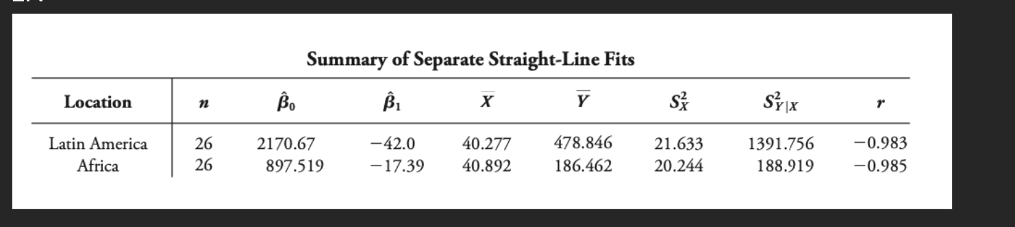
Comment on the validity of homogenous variance assumption for these data.

The residual variances S² from the textbook table shows that the S² for Latin America is 21.633 and the S² for Africa is 20.

Determining the dose-response straight lines

Y^=B0+B1X

Y^male=14.178+14.825*X

Y^female=15.656+12.735*X

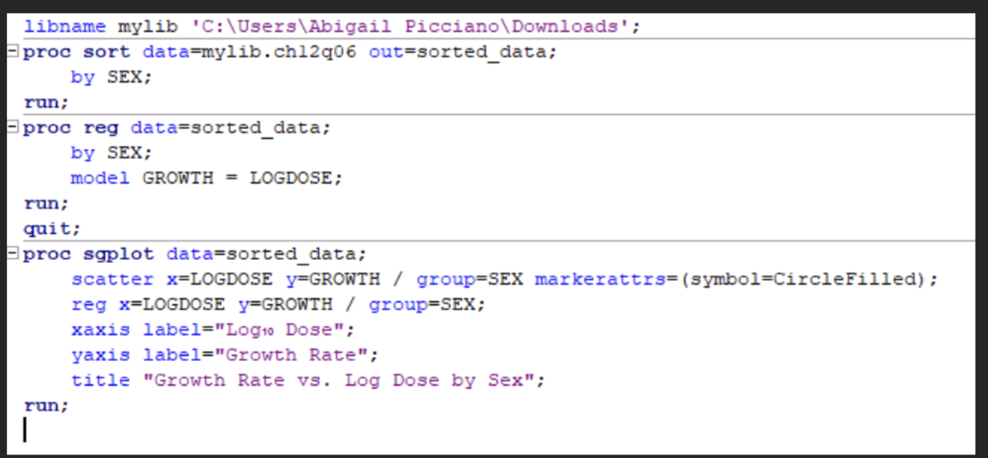
SAS code to graph the dose response lines

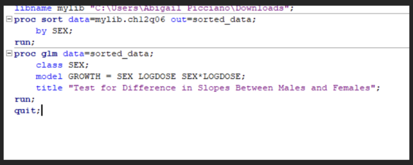
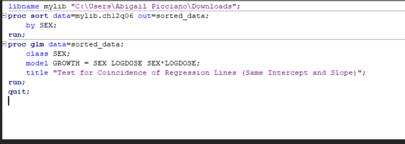
SAS code for testing the difference in slopes between Males and Females

The p-value for the interaction the LOGDOSE * SEX is 0.4327, therefore there is no statistically significant difference in slopes of the regression lines for males and females. The data does not provide sufficient evidence to conclude that the dose-response relationship differs by sex.

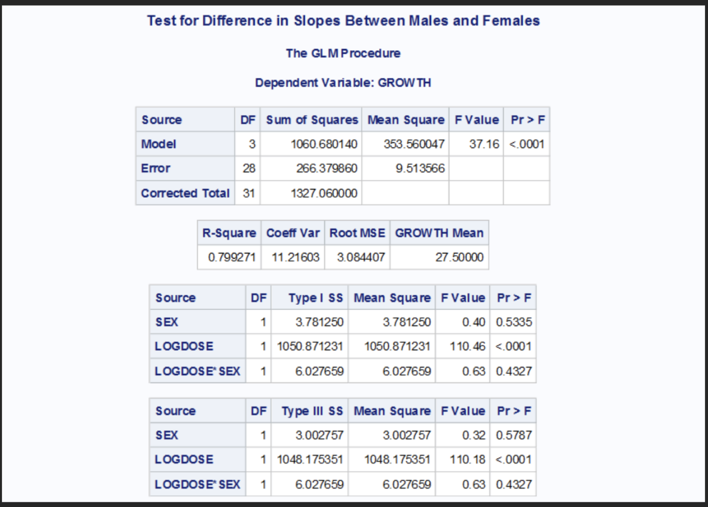
Test for coincidence of the two straight lines

H0: The two lines are coincident (same slope and same intercept)

HA: The two lines differ (either slope or intercept or both)

The p-value is 0.5787 which is not significant at the alpha level of 0.01 and the p-value for LOGDOSE*SEX is 0.4327 which is also not significant at the alpha level of 0.01 therefore we fail to reject the null hypothesis. The data provides significant evidence that the regression lines for both males and females differ in either slope or intercept at the 99% confidence level. This means that the regression line of the two sexes are coincident suggesting a shared dose-response relationship.

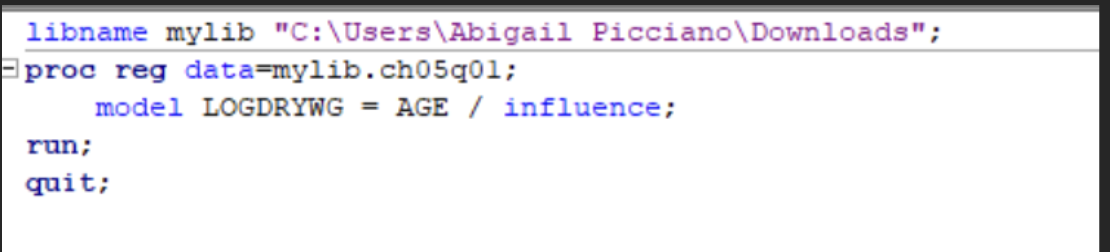
SAS code for examining a plot of studentized or jacknife residuals versus the predicted values.

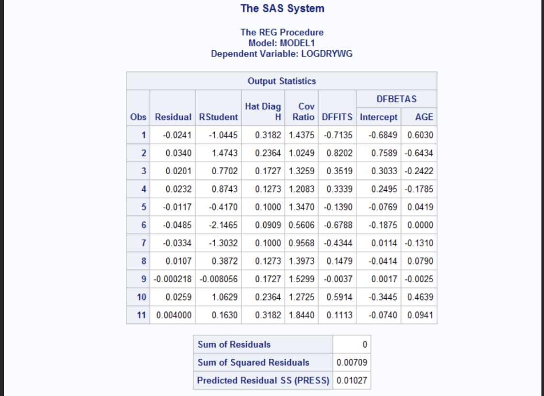
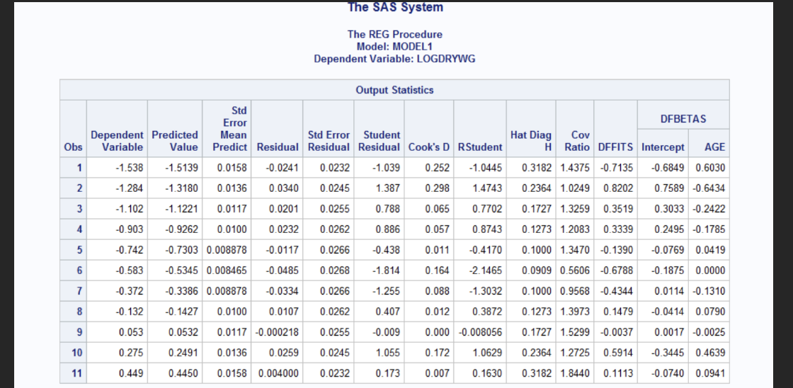
The Rstudent which represented the studentized residuals account for the variance of each observation. These values range from -2.1465 (observation 6) to 1.4743 (observation 2). Since observation 2 exceeded +-2 it may indicate a potential outlier. Hat Diag H which is Leverage values range from 0.09 to 0.3182 which are within the acceptable range. For DFFITs it assesses how much an observation influences its fitted value. The general cutoff: DFFITs> 2square root p/n= 0.85 for small samples. The observations 1 and 2 have values close in value with observation 1= -0.7135 and observation 2= 0.8202 nearly crosses the threshold and may require further investigation. DFBETAs are measures that impact the observation on individual regression coefficients. Value>|1| may indicate a potential influence on that coefficient. In the output, all DFBETAs for the intercept and AGE are |1|, so no excessive influence is evident.  

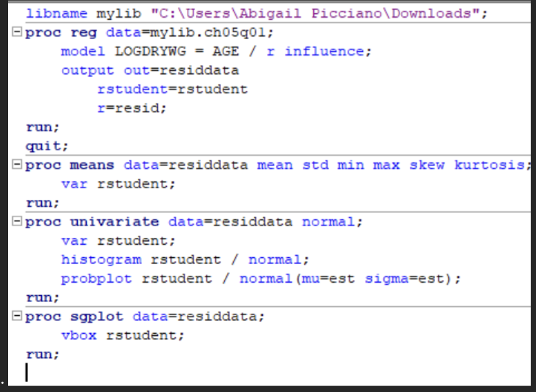
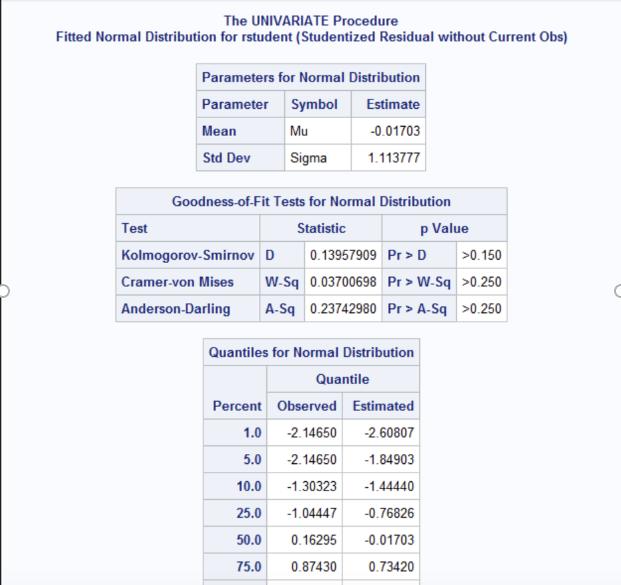
SAS code for examining numerical descriptive statistics, histograms, box and whisker plots, and normal probability plots of jacknife residuals. Is the normality assumption violated?

The goodness of fit tests including the Kolmogorov-Smirnov test D= 0.1396, p>0.150, Cramer-von Mises (W-sq= 0.0370, p>0.250) and Anderson-Darling (A-Sq= 0.2374, p>0.250) tests all show non-significant p-values suggesting no evidence to reject the null hypothesis of normality. The Q-Q plot shows that the studentized residuals lie close to the diagonal line, indicating a good fit for the normal distribution. The boxplot shows symmetric distribution with no extreme outliers, and the spread of the residuals is balanced around the median supporting the normality assumption. The histogram of studentized residuals closely resembles a bell-shaped curve while there is slight skewness in the overall shape with the normal curve. In the descriptive stats, the mean of the residuals is approximately –0.017 which is close to zero and the standard deviation is about 1.11 which is consistent with normality expectations. Overall, there is no evidence of serious violations of the normality assumption. Therefore, no additional remedies.  

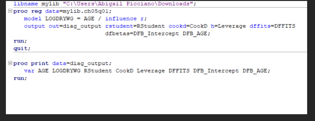
SAS code for examining outlier diagnostics including cook’s distance, leverage statistics, and jacknife residuals. Identify any potential outliers

Studentized (Jacknife) Residuals: All the values fall within +-3 with a range of –2.15 to 1.47 suggesting no major outliers based on the residuals alone. For cooks the distance the maximum is 0.298 observation 2, which is below the influence threshold of 0.364 (4/n). Thus, there are no observations highly influential on this measure. The leverage Hat values the highest is 0.3182 (observation 1) which is below the typical cutoff of 2p/n= 0.36 for 2 parameters and 11 observations with no high leverage points detected. The DFFITS observation 2 has the highest DFFITs at 0.8202 slightly above the suggested threshold. This may indicate moderate influence, but it’s isolated. The DFBETAS of all values fall well below +- 1 indicating no single observation has undue influence on the regression coefficients.   

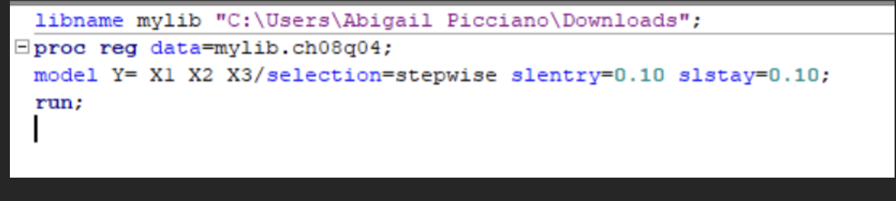
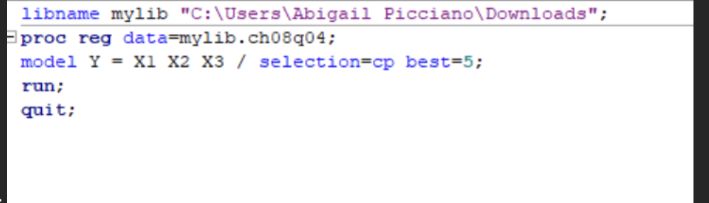
SAS code for stepwise approach, the best regression model relating homocide rate (Y), population size (X1), percentage families with income less than $5,000 (X2) and unemployment rate (X3)

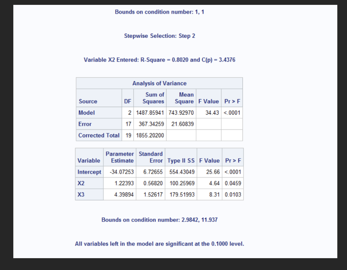
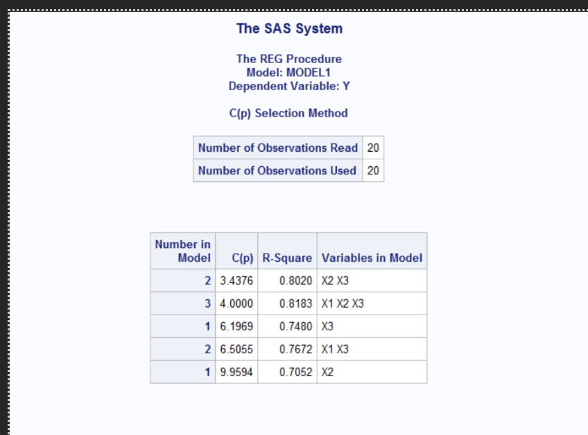
The stepwise regression selected X3 and X2 for the final model. X3 was entered first, explaining 74.8% of the variance p<0.0001 followed X2 which added 5.4% more explanatory power p=0.0459. The final model had an R^2 of 0.8020 and C(p) value of 3.4376 indicating a good fit. Both predictors are statistically significant, and no other variables met the entry criterion at the 0.10 level.  

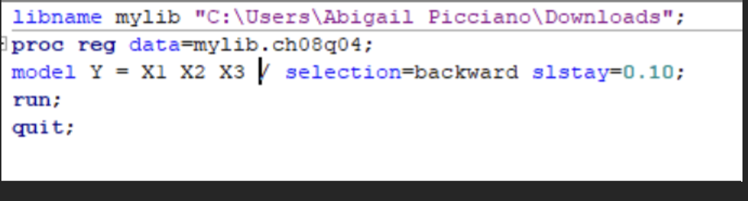
SAS code for the Backward approach

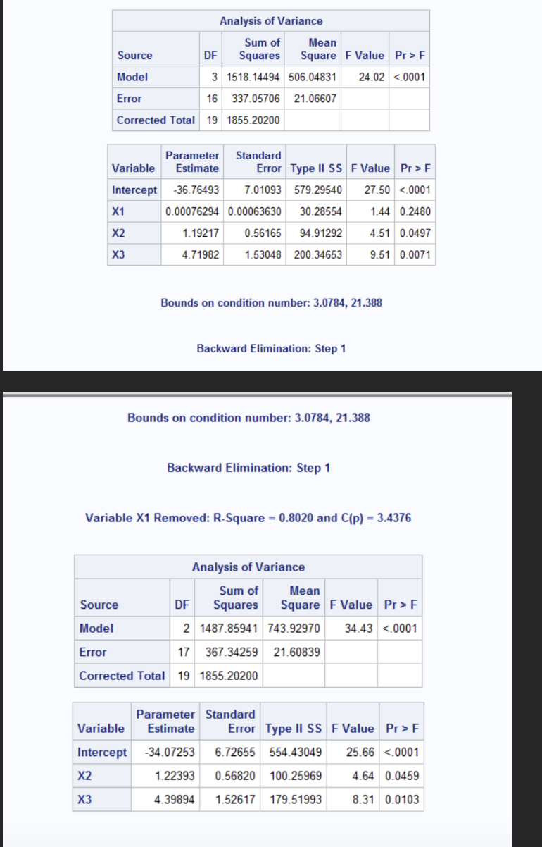
Backward elimination began with all three predictors of X1, X2, and X3 in the model. The initial model has an R^2 of 0.8183 and C(p) of 4.0000 indicating a strong overall fit. In step 1, the variable X1 was removed because it was not statistically significant at p=0.2480 and contributed little to the model (partial R^2= 0.0163). After removing X1, the model R^2 decreased slightly to 0.8020 and C(p) dropped to 3.4376. The final model retained X2 and X3, both of which were statistically significant at the 0.10 level.  

SAS code for all possible regression

Based on all regression approaches using Mallow’s Cp the best model at alpha=0.10  is the model that includes X1 (income under 5k) and X3 (unemployment rate). This model has a good R^2 fit of 0.8020 and Cp value of 3.44 close to the number of predictors indicating that it is a well balanced model.  

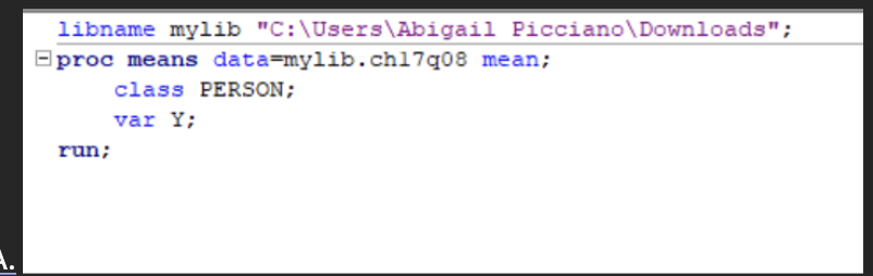
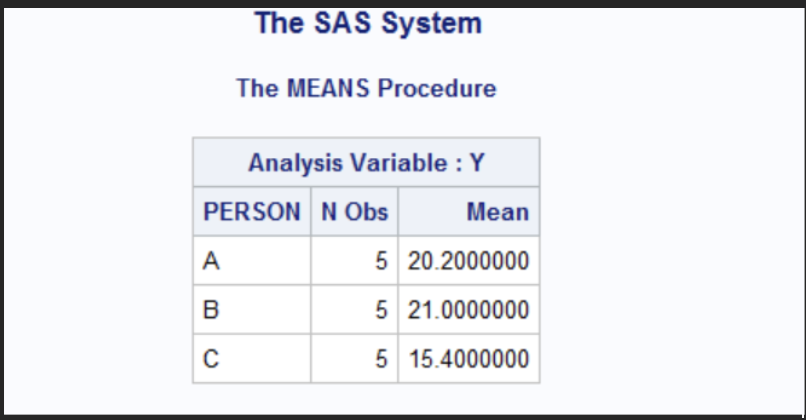
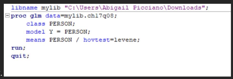
SAS code for determining the mean score for each person

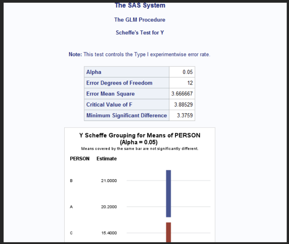
For person A the mean is 20.2, person B the mean is 21.0 and person C the mean is 15.4. Meaning person B had the highest on average correct answers following person A closely and then after Person C had the lowest on average correct answers.  

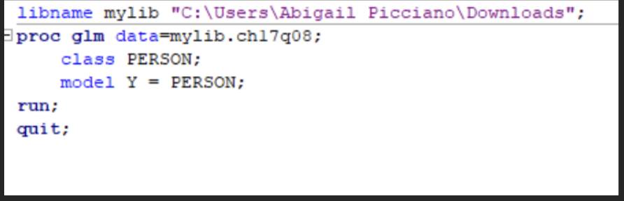
Test whether the three persons have significantly different ESP ability

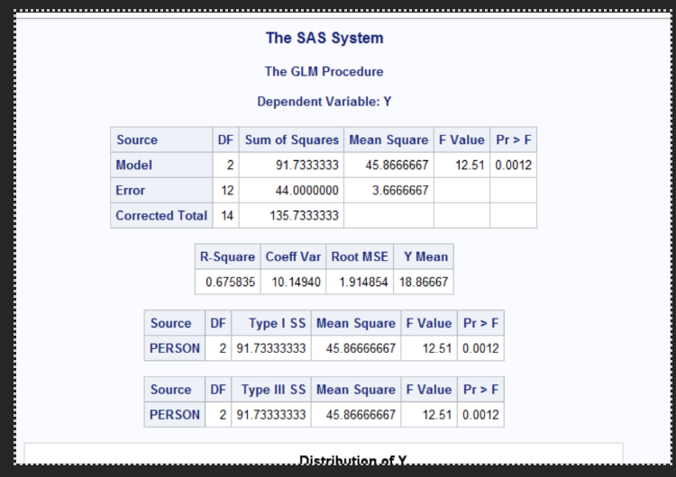
Since p= 0.0012 <0.05 we reject the null hypothesis meaning there is strong statistical evidence that at least one person’s ESP performance differs significantly from the others.  

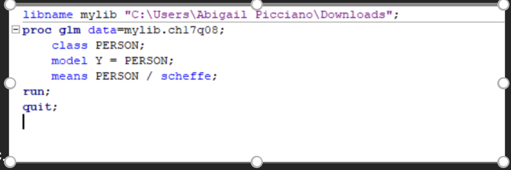
Carry out Scheffe’s multiple comparison procedure to determine which pairs of persons, if any significantly differ in ESP ability

The Mean square error was 3.6667 which means there is a significantly different means. In this test, person C differs significantly from person A and B. However, person A and B do not differ significantly from each other.  

On the basis of the results from parts b and c, can one conclude there any of these persons have statistically significant ESP ability

Based on part b and c, we can conclude that the three individuals differ significantly in ESP performance, particularly that Person C performed significantly worse than Persons A and B. However, these results do not provide evidence that any individual has ESP ability, because the test only compares participants against each other, not against a chance level benchmark. To establish statistically significant ESP ability, we would need to test whether each person’s mean score is significantly above the chance level.  

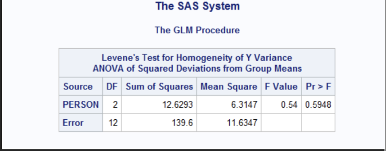
What basic ANOVA assumptions might be violated here?

Normality might be violated since each group contains only 5 observations. Small sample sizes limit the ability to formally test or visually assess normality through histograms, Q-Q plots, and the central limit theorem does not fully apply here. Independence is met as the observations of the ESP scores for each person are on different days and appear to be independent since they are collected across separate testing days for everyone. There is no indication of dependence or repeated measures, so this assumption is reasonably met. Homogeneity of variances was tested using Levene’s test for equality of variances. The result in the output was F= 0.54 and p= 0.5948. Since the p value is greater than 0.05 we fail to reject the H0 of equal variances.  

Assuming that there is a randomized block design what are the blocks and what are the treatments?

The treatments are the three genotypes of silkworms being studied. HOM= homozygous, HET= Heterozygous and WLD: Wild-type 

Each genotype represents a distinct treatment condition whose effect on cocoon body length is being evaluated.  

The blocks are the five laboratory sites from site 1 through site 5 where the measurements were taken.   

Why do you think randomized block analysis is appropriate or inappropriate for this experiment?

A randomized block analysis is appropriate for this experiment because there is a clear potential source of variability across the five laboratory sites. Factors such as differences in equipment, environmental conditions, or handling procedures at each site could affect the measured cocoon lengths, even if the silkworm genotype remains the same. By treating the site as a blocking factor, we can account for site-to site variability and focus the analysis on the true effect of the genotype on cocoon length. Blocking improves precision of the experiment by reducing the residual error and controlling nuisance variance. 

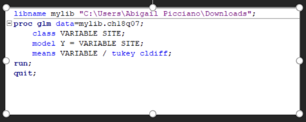
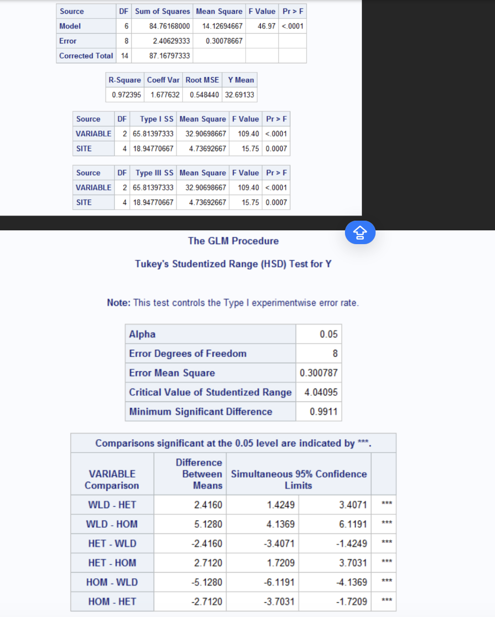
Carry out an appropriate analysis for this data for this experiment and state your conclusions.

Hypotheses:  

Main treatment effect (genotype) 

H0: The mean cocoon lengths are equal for HOM, HET, and WLD.  

H1: At least one genotype has a different mean cocoon length  

 

Post hoc comparisons 

H0: There is no difference in mean length between each pair of genotypes.  

H1: The mean cocoon lengths for each pair are significantly different.  

 

The results showed that genotype had a statistically significant effect on cocoon length F (2, 8) = 109.40 p<0.0001). Additionally, the blocking factor (Site) was also statistically significant with F (4, 8) = 15.75 p=0.0007) confirming that accounting for site-to-site variation was appropriate and necessary.  Post hoc comparisons using Tukey’s HSD test showed that all pairwise differences between genotype were statistically significant at the 0.05 level. With Wild type (WLD) silkworms had significantly larger cocoons than both heterozygous (HET) and homozygous (HOM) genotypes with a mean difference of 5.1280mm between WLD and HOM. HET silkworms also had a significantly larger cocoon than HOM with a mean difference of 2.71